Modeling
To run this tutorial, all data files should be available in in the directory examples/examples_modeling_tutorial/model_data/.
[1]:
%matplotlib inline

import os
import numpy as np
import math
import time

from matplotlib import pyplot as plt
from matplotlib import rcParams
from matplotlib import gridspec
from matplotlib import cm

rcParams['text.usetex'] = False
rcParams['font.size'] = 14.0

import xpsi

from xpsi.global_imports import gravradius, _2pi
from xpsi.utilities import PlottingLibrary as XpsiPlot
/=============================================\
| X-PSI: X-ray Pulse Simulation and Inference |
|---------------------------------------------|
|                Version: 3.3.0               |
|---------------------------------------------|
|      https://xpsi-group.github.io/xpsi      |
\=============================================/

Imported emcee version: 3.1.6
Imported PyMultiNest.
Imported UltraNest.
Imported GetDist version: 1.5.3
Imported nestcheck version: 0.2.1
Let’s build a generative model for the data; first we build a callable object for likelihood evaluation, and then we build a callable object for prior-density evaluation.
En route, we will explain why various software design choices were made during development. In some cases the conventions defined are not necessarily important for future development and indeed we expect them to be redesigned.
Likelihood
If you have not yet read the likelihood overview, it is advisable to do so now, or refer to a paper such as Riley et al. (2019).
The parameter space
In order to implement an X-PSI likelihood function it is first necessary to define an underlying model parameter space. In general the parameter space is \(\mathbb{R}^{d}\), where \(d\in\mathbb{N}\) is the total number of free model parameters. Each free parameter is an instance of the Parameter class. We also support fixed (or frozen) variables and derived variables that are deterministic functions of other variables (notably, free parameters).
In X-PSI we build upon a base class representing a ParameterSubspace. To construct an X-PSI model a set of objects are defined which derive from this parameter subspace, and it is the union of these objects that forms both the global model parameter space, and a set of methods and attributes for evaluation of a parametrised sampling distribution of the data at the vector \(\mathcal{D}\), conditional on a vector of model parameter values.
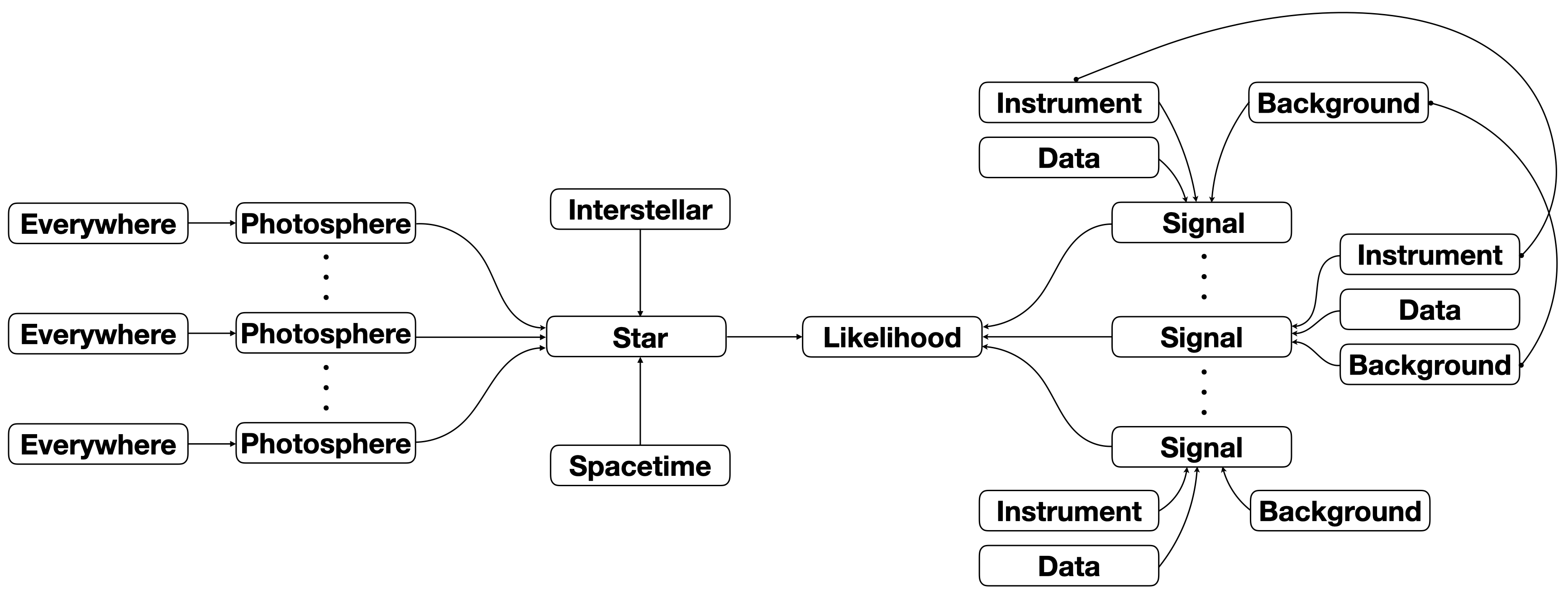
Our aim is to construct a callable likelihood object to feed as a callback function to a posterior sampler and a posterior integrator. We illustrate this object in the diagram below; all nodes in the diagram below represent objects (instances of some class). In some cases there are multiple instances of a particular class, in other cases there is only a single instance of a particular class. Moreover, a subset of these classes inherit from (subclass)
ParameterSubspace, because instances of these classes are objects with a parameter subspace and a collection of methods with instructions for handling parameter vectors in that subspace (methods and attributes to, e.g., calculate and store some derived quantities of the underlying theory/model respectively for likelihood evaluation).
[2]:
from IPython.display import Image
Image("./_static/oop_modelling_diagram_v1.png")
[2]:
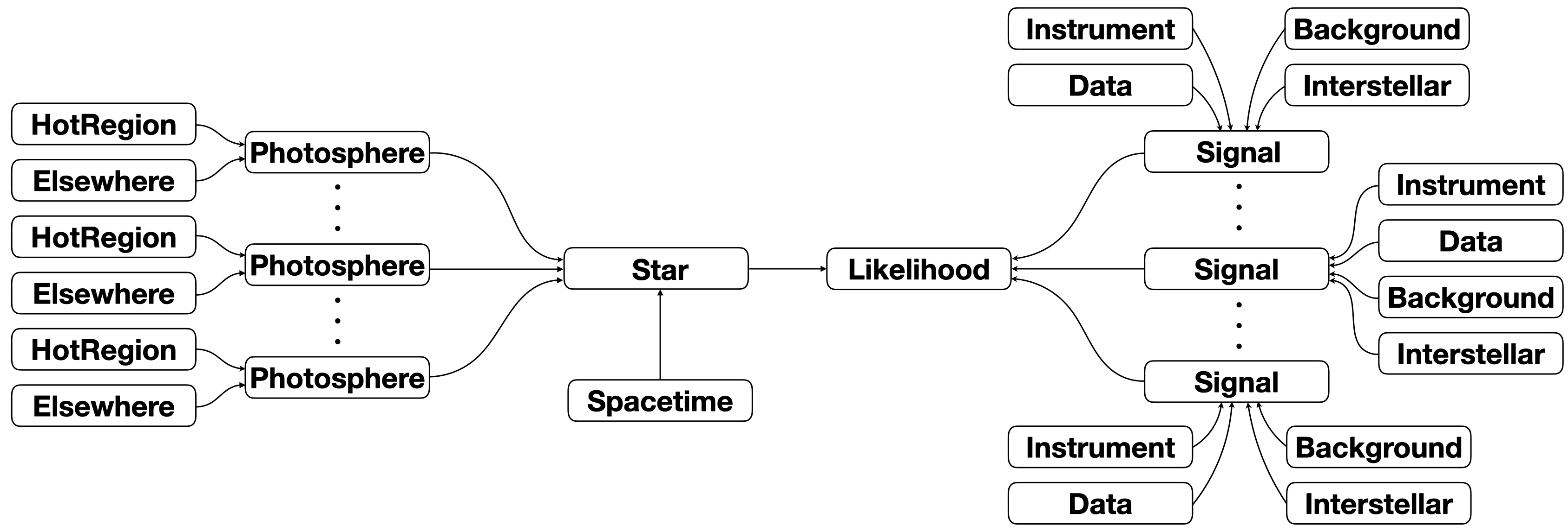
The arrows in the diagram denote an object that is stored as an attribute of another encapsulating (a reference to) another object. When a call is processed to evaluate the likelihood given a vector of model parameter values, encapsulating objects get attributes (magically including method calls) of the wrapped objects. The likelihood call results in a cascade of attribute lookups by objects higher in the hierarchy to those lower in the hierarchy. An arguably powerful aspect of the
implementation is the merging of parameter subspaces when references to two or more subspaces are encapsulated with an object higher in the hierarchy. This permits parameters to be accessed via Python container __getitem__ and __setitem__ magic on any object (deriving from ParameterSubspace) that encapsulates references to them.
We will now briefly describe the purpose of each object above which is encapsulated by the callable likelihood object (Likelihood in the diagram to denote the name of the class of which it is an instance). Note the use of the term abstract base class, which means that a user is required to subclass, and thereby provide a concrete implementation of some functionality specific to their model. Some source code classes are concrete classes that can be instantiated directly.
A
Starinstance derives from theParameterSubspaceclass. It represents the model star. The objects it encapsulates also derive from theParameterSubspaceclass.A
Spacetimeinstance derives from theParameterSubspaceclass. It represents the ambient Schwarzschild spacetime solution.A
Photosphereinstance derives from theParameterSubspaceclass. It represents a radiation field on a 2-surface embedded in a spacelike hypersurface of that ambient spacetime. There can be multiplePhotosphereinstances perStarinstance, naturally representing snapshots in time that are assumed to be adequate approximations for some natural number of stellar rotations. Note that the dimensionality of the parameter space grows linearly, however, so in practice this approximation to time evolution is intended for simulation and data synthesis.A
HotRegioninstance derives from theParameterSubspaceclass. It represents a radiatively intense region: e.g., a “circular hot-spot” in the photosphere (the surface radiation field). Alternatively, aTwoHotRegionsobject that derives fromHotRegion, or aHotRegionsobject that encapsulates references to two or moreHotRegioninstances, is used.An
Elsewhereinstance derives from theParameterSubspaceclass. The represents the surface radiation field exterior to the hot region.An
Everywhereinstance derives from theParameterSubspaceclass. The represents the surface radiation field everywhere, and cannot be used in conjuction withHotRegioninstances andElsewhereinstances.
A
Signalinstance derives from theParameterSubspaceclass, and is itself an abstract base class. A signal is defined as a subset \(\mathcal{D}_{i}\subseteq\mathcal{D}\) of the dataset with a parametrised sampling distribution dependent on an incident specific flux signal generated by a particularPhotosphereinstance. There can thus be multipleSignalinstances.A
Datainstance does not derive from theParameterSubspaceclass, and is a concrete class. It is a container for the data subset \(\mathcal{D}_{i}\subseteq\mathcal{D}\).An
Instrumentinstance derives from theParameterSubspaceclass, and is a concrete class. It represents the model instrument for transforming incident specific flux signals into a structure which directly enters the parameterised sampling distribution of \(\mathcal{D}_{i}\).An
Interstellarinstance derives from theParameterSubspaceclass, and is itself an abstract base class. It represents a model for physical interstellar radiation-matter interaction processes which modify the surface radiation field during propagation to the instrument.A
Backgroundinstance derives from theParameterSubspaceclass, and is itself an abstract base class. It represents a model for the background radiation field incident on the instrument.
The purpose of invoking the object-oriented paradigm here is to organise a non-trivial likelihood evaluation algorithm in a logical, flexible, and extensible manner by identifying groups of mathematical structures which can be considered as belonging to some more abstract object with some physical and/or statistical meaning, and modularising them in classes.
We use a dynamic and expressive high-level language to organise this computation, allowing both calls low-level library routines where necessary to improve calculation speed, and straightforward communication between our problem-specific code and other more general open-source software libraries (in particular, statistical sampling software).
As stated above, for each of these objects which derive from the ParameterSubspace class, their parameter subspaces are merged into a higher-dimensional space when referenced by an object higher in the hierarcy. As an example, a HotRegion instance and an Elsewhere instance each have an associated parameter subspace, and those are merged to form most of the dimensions of the parameter space associated with a Photosphere instance.
Note that one can in principle utilise a given object multiple times. An example would be the use of the same Instrument object or Interstellar processes object for constructing multiple Signal objects, although this might result in too many parameter dimensions for a problem to be tractable. On another level, the instruments might reference some of the same Parameter objects, but themselves be distinct objects, each passed to a distinct Signal object. In the diagram below we
illustrate a tied relationship between some objects with connecting lines: this could mean the tied objects are the same object, or that the objects share some parameters, or that properties of one are derived from the free parameters of another.
[3]:
Image("./_static/oop_modelling_diagram_v2.png")
[3]:
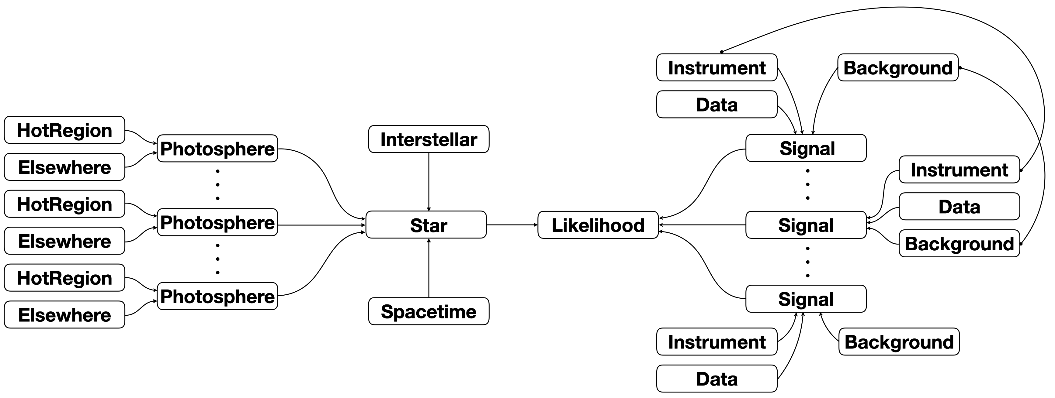
In this case, the tied objects represent physical systems or processes exisiting at different times, but some behaviour is shared. Note that we also assumed that the Interstellar processes are time-invariant and thus moved the object over to connect to the Star itself; the source code is not structured quite in this way, but achieves the same if an Interstellar process object is time-invariant. The Data objects are never parametrised and thus are not tied in the sense discussed
above.
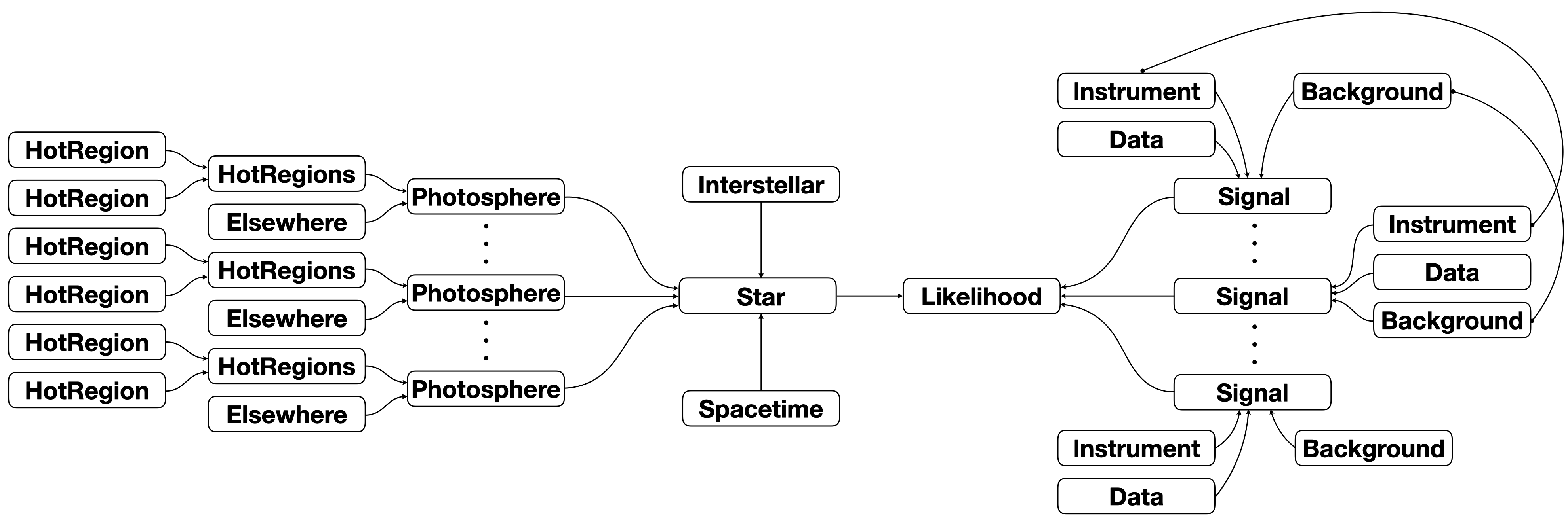
Another example might be supplying the same hot-region radiation field parameters to two disjoint hot regions that simultaneously occupy a subset of the stellar surface. In this case the Parameter objects referenced in the HotRegion objects would be shared. Another way to achieve the same effect is to define parameters of one hot region as derived from those of the other hot region. Both methods would achieve the same goal, but would be implemented differently. The latter is more
flexible and thus more powerful. More extensive examples of this paradigm are given in a separate tutorial.
If there are instantaneously multiple disjoint surface hot regions, the model object hierarchy diagram would more accurately be rendered as:
[4]:
Image("./_static/oop_modelling_diagram_v3.png")
[4]:
If there are multiple instances of the Photosphere class, and multiple instances of the Signal class with a one-to-one mapping, the parameter set would assume the following form:
coordinate spin frequency
(rotationally deformed) gravitational mass
coordinate equatorial radius
distance from Earth
inclination of Earth to stellar rotation axis
photosphere_1(non-optional):coordinate rotation frequency of a mode of radiative asymmetry assumed to generate the observed pulsations
subvector of geometric hot-region parameters (e.g., spot centre colatitude, spot angular radius, and so on) and a parameter controlling the surface local-comoving-frame radiation field within the region boundaries
(optional) subvector of additional parameters controlling the surface local-comoving-frame radiation field within the hot-region boundaries (e.g., pertaining to ionisation degree or composition)
(optional) subvector of parameters controlling the surface local-comoving-frame radiation field outside the hot-region boundaries
subvector of fast parameters for the phases of the hot region(s) relative to some fiducial phase
\(\ldots\)
photosphere_n(optional):coordinate rotation frequency of a mode of radiative asymmetry assumed to generate the observed pulsations
subvector of geometric hot-region parameters (e.g., spot centre colatitude, spot angular radius, and so on) and a parameter such as an effective temperature controlling the surface local-comoving-frame radiation field within the region boundaries
(optional) subvector of additional parameters controlling the surface local-comoving-frame radiation field within the hot-region boundaries (e.g., pertaining to ionisation degree or composition)
(optional) subvector of parameters controlling the surface local-comoving-frame radiation field outside the hot-region boundaries
subvector of fast parameters for the phases of the hot region(s) relative to some fiducial phase
signal_1(non-optional):(optional) subvector of fast nuisance parameters associated with interstellar processes
(optional) subvector of fast nuisance parameters associated with instrument response
(optional) subvector of fast nuisance parameters associated with background processes
\(\ldots\)
signal_n(if matchingphotosphere_n):(optional) subvector of fast nuisance parameters associated with interstellar processes
(optional) subvector of fast nuisance parameters associated with instrument response
(optional) subvector of fast nuisance parameters associated with background processes
where \(\forall i\in[1,n]\) photosphere_i and signal_i share an identification tag.
Most model parameters that are not associated with Signal instances are considered slow parameters; see the interlude below for definition of slow and fast. An example of a slow parameter is the gravitational mass, whilst examples of fast parameters are the initial phase of the photosphere and the distance (from Earth) to the star.
Yet another paradigm is that the same signal yielded by integrating over the photosphere is operated on by multiple instruments (on different telescopes or the same telescope, or some on one telecope and others on other telescopes), and because these instruments are synergystic probes of the physical signal-generating process, we aim to jointly model the data from those instruments. This can be executed as follows:
[5]:
Image("./_static/oop_modelling_diagram_v4.png")
[5]:
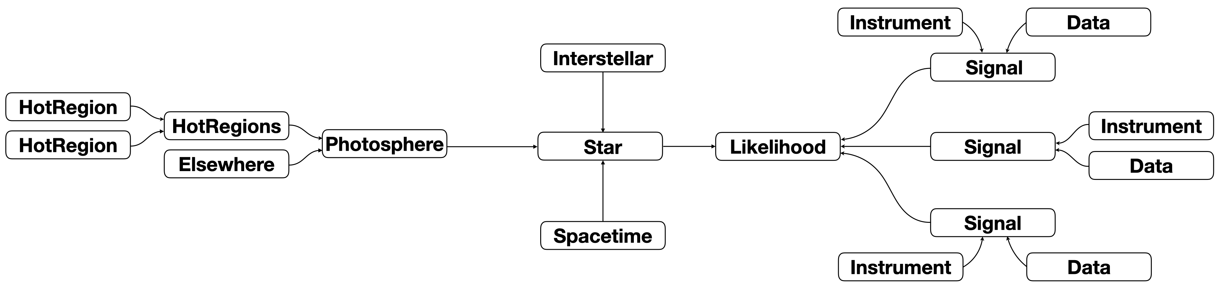
Here the signal from integrating over the image of the Photosphere instance is relayed to all Signal instances for instrument operation and likelihood function calculation. The signal relayed is always encapsulated by a 2D NumPy array with photon energy increasing with row (zeroth dimension) and phase increasing with column (first dimension). Even if an integrator (extension module) is called that assumes time-invariance of the image of the Photosphere and thus returns a single
spectrum, that spectrum is encapsulated by a 2D NumPy array. Specifically, an Elsewhere instance returns a spectrum which is added to the spectrum at each phase generated by the associated HotRegion(s) instance. The user can then completely phase-average the signal (thus generating a single spectrum) for comparison to an instrument whose registered (and pre-processed) data is a spectrum. For instruments that register time-resolved data, the user will usually integrate the signal phase
intervals (bins) for likelihood function evaluation. The phase-resolved and phase-averaged data can be jointly modeled.
Finally, one can use Everywhere instances to model the surface radiation field everywhere, but these instances cannot be used in conjuction with HotRegion instances nor Elsewhere instances to constitute the same Photosphere instance. An example of this paradigm is as follows:
[6]:
Image("./_static/oop_modelling_diagram_v5.png")
[6]:
Note that here we chose to return to the notion of time-evolution between Photosphere instances, instead of using multiple Signal intances operating on one Photosphere instance.
Interlude: fast and slow parameters
A subset of model parameters are slow because varying those parameters requires likelihood re-evaluation, and the compute time required to perform that re-evaluation is slow relative to re-evaluation when varying only a distinct subset of the model parameters: the fast parameters. In general there can be multiple subsets of parameters forming a speed hierarchy; see A. Lewis, “Efficient sampling of fast and slow cosmological parameters” (arXiv:1304.4473).
X-PSI, during developement, supported the use of the nested sampler PolyChord, whose internals require that parameters forming a speed hierarchy are ordered in subsets (or blocks) from slow to fast in an array passed to a likelihood callback function (if one wishes to exploit a speed hierarchy that is). Thus the ordering of an array of parameter values passed to a general instance of the Likelihood class was of crucial importance. During
development, we opted to support the nested sampler MultiNest instead based on the nature of the sampling problem (dimensionality and likelihood evaluation expense).
However, until X-PSI v0.3, a convention for parameter ordering for likelihood evaluation was imposed, with two basic speed grades. In v0.3, however, we do not adhere to a speed hierarchy for lack of an application at present, although with some added sophistication this can be supported.
Data
For the analysis in this notebook we consider all data \(\mathcal{D}\) to be drawn from a joint sampling distribution whose dependency on slow model source parameters is expressed in terms of a single pulse signal. The justification for such an assumption is that we are performing parameter estimation given a synthetic data set for a model pulsar with a stable (effectively non-evolving) surface radiation field, with any quasi-periodicity arising solely from relative orbital motion of source and telescope. The synthetic data is intended to emulate detection of photons over a long observing run, after which the photon incidence events are phase-folded during a pre-processing phase.
This parameter estimation excercise is not blind: we know the parameter values injected to generate the synthetic dataset we will later load into a custom container.
We do not need to subclass data container, but you can if you wish. X-PSI is designed this way because there is a clear common usage pattern that can be concretely implemented whilst preserving the freedom and the scope of applicability of the source code. The container instance will be available as an underscore instance method of Signal, and thus available in a derived class where we will later write code for likelihood evaluation.
Hereafter we will write our custom derived classes in the notebook itself, but in practice it is best if your derived classes are written in distinct modules within a project directory, so they can be imported by a script for use with an MPI command within a shell (because in general we want to exploit parallelism for expensive likelihood evaluations).
Let us load a synthetic data set that we generated in advance, and know the fictitious exposure time for:
[7]:
settings = dict(counts = np.loadtxt('../../examples/examples_modeling_tutorial/model_data/example_synthetic_realisation.dat', dtype=np.double),
                channels=np.arange(20,201),
                phases=np.linspace(0.0, 1.0, 33),
                first=0, last=180,
                exposure_time=984307.6661)

data = xpsi.Data(**settings)
Setting channels for event data...
Channels set.
For real data, the X-ray telescope processing pipeline usually result in an event file (EVT) or spectrum (PHA). X-PSI can fit both, but there is not timing information in PHA file. Those can be loaded with xpsi.Data.load(file_path,n_phases=32, channels=None, phase_column='PULSE_PHASE', channel_column='PI') where :
file_pathpoints to an EVT or PHA filen_phaseis the number of phase bins ro divide the data into if this is an EVT filechannelsgives list of channels to extractphase_columnis the column to take the phase values from if this is an EVT filechannel_columnis the column to take the channel values from if this is an EVT file
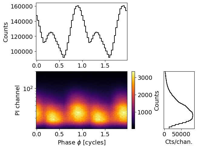
Let’s take a look at the data that we aim to model. We can plot it with a built in function :
[8]:
fig, axs = data.plot( dpi=100 , colormap='inferno' , num_rot=2)
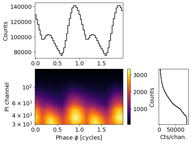
We can trim it and replot it
[9]:
data.trim_data(min_channel=30, max_channel=180 )
fig, axs = data.plot( dpi=100 , colormap='inferno' , num_rot=2)
Trimming event data...
Event data trimmed.
[10]:
# Let's go back to the first configuration
data = xpsi.Data(**settings)
Setting channels for event data...
Channels set.
Instrument
We require a model instrument object to transform incident specific flux signals into a form which enters directly in the sampling distribution of the data.
[11]:
class CustomInstrument(xpsi.Instrument):
    """ A model of the NICER telescope response. """

    def __call__(self, signal, *args):
        """ Overwrite base just to show it is possible.

        We loaded only a submatrix of the total instrument response
        matrix into memory, so here we can simplify the method in the
        base class.

        """
        matrix = self.construct_matrix()

        self._folded_signal = np.dot(matrix, signal)

        return self._folded_signal
Let’s construct an instance.
[12]:
NICER = CustomInstrument.from_ogip_fits(RMF_path='nicer_20170601v003.rmf',
                                        ARF_path='nicer_20170601v005.arf',
                                        datafolder='../../examples/examples_modeling_tutorial/model_data')
Loading instrument response matrix from OGIP compliant files...
Triming the response matrix because it contains columns with only 0 values.
 Now min_channel=9 and max_channel=1500
Setting channels for loaded instrument response (sub)matrix...
Channels set.
An empty subspace was created. This is normal behavior - no parameters were supplied.
Response matrix loaded.
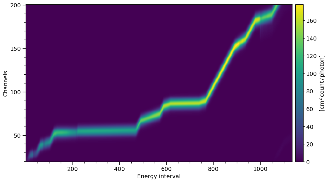
The NICER response matrix is non-diagonal because some energy ranges are oversampled.
[13]:
energy_inputs = np.arange(1,len( NICER.energy_edges)+1)-0.5
channels = NICER.channel_edges * 100 - 0.5

rmf_plot = XpsiPlot.plot_rmf(matrix=NICER.matrix,
                             x=energy_inputs,
                             y=channels,
                             xlabel='Energy interval',
                             ylabel='Channels'
                            )

XpsiPlot.veneer((200, 1000), (50, 100), rmf_plot)
The response is large, let’s trim it for plotting
[14]:
NICER.trim_response(min_channel=20, max_channel=200, tolerance=1e-5)
print( NICER.matrix.shape )

# Update the x and y arrays for the plot
energy_inputs = np.arange(1,len( NICER.energy_edges)+1)-0.5
channels = NICER.channel_edges * 100 - 0.5

rmf_plot = XpsiPlot.plot_rmf(matrix=NICER.matrix,
                             x=energy_inputs,
                             y=channels,
                             xlabel='Energy interval',
                             ylabel='Channels'
                            )
XpsiPlot.veneer((50, 200), (10, 50), rmf_plot)
Trimming instrument response...
Setting channels for loaded instrument response (sub)matrix...
Channels set.
Triming channels of the response matrix because a smaller channel range has been requested.
 Now min_channel=20 and max_channel=200
Triming energy inputs of the response matrix with tolerance 1e-05.
 Now min_energy=0.10000000149011612 and max_energy=12.930000305175781
Instrument response trimmed.
(181, 3064)
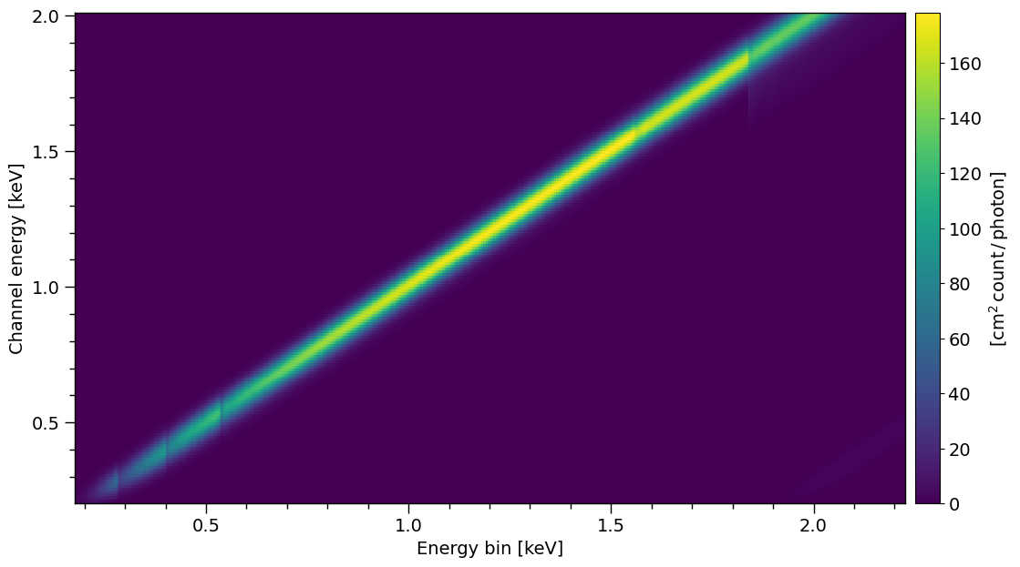
Plotting now with the energy values
[15]:
rmf_plot = XpsiPlot.plot_rmf(matrix=NICER.matrix,
                             x=NICER.energy_edges,
                             y=NICER.channel_edges,
                             xlabel='Energy bin [keV]',
                             ylabel='Channel energy [keV]',
                            )
XpsiPlot.veneer((0.1, 0.5), (0.1, 0.5), rmf_plot)
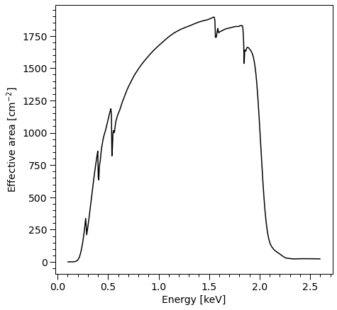
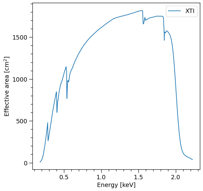
Summed over channel subset \([20,200]\):
[16]:
arfplot = XpsiPlot.plot_arf([NICER])
XpsiPlot.veneer((0.1, 0.5), (100, 500), arfplot)
Signal
We can now combine the dataset and model instrument into a Signal object. The source code for this class has methods and attributes which simplify communication between the aforementioned model objects and another object representing our model star (created below). The surface radiation field of the model star is integrated over based on energies relayed from a Signal object based on the properties of the instrument and the dataset (which are tightly coupled).
We are forced to inherit from Signal and write a method that evaluates the logarithm of the likelihood conditional on a parametrised sampling distribution for the data. There is much freedom in constructing this sampling distribution, so the design strategy for X-PSI was to leave this part of the modelling process entirely to a user, guided by a number of examples. The only condition for applicability is that the sampling distribution of the data (or of each subset) can be written in terms of a set of single count-rate pulses.
[17]:
from xpsi.likelihoods.default_background_marginalisation import eval_marginal_likelihood
from xpsi.likelihoods.default_background_marginalisation import precomputation

class CustomSignal(xpsi.Signal):
    """

    A custom calculation of the logarithm of the likelihood.
    We extend the :class:`~xpsi.Signal.Signal` class to make it callable.
    We overwrite the body of the __call__ method. The docstring for the
    abstract method is copied.

    """

    def __init__(self, workspace_intervals = 1000, epsabs = 0, epsrel = 1.0e-8,
                 epsilon = 1.0e-3, sigmas = 10.0, support = None, **kwargs):
        """ Perform precomputation.

        :params ndarray[m,2] support:
            Prior support bounds for background count rate variables in the
            :math:`m` instrument channels, where the lower bounds must be zero
            or positive, and the upper bounds must be positive and greater than
            the lower bound. Alternatively, setting the an upper bounds as
            negative means the prior support is unbounded and the flat prior
            density functions per channel are improper. If ``None``, the lower-
            bound of the support for each channel is zero but the prior is
            unbounded.

        """

        super(CustomSignal, self).__init__(**kwargs)

        try:
            self._precomp = precomputation(self._data.counts.astype(np.int32))
        except AttributeError:
            print('Warning: No data... can synthesise data but cannot evaluate a '
                  'likelihood function.')
        else:
            self._workspace_intervals = workspace_intervals
            self._epsabs = epsabs
            self._epsrel = epsrel
            self._epsilon = epsilon
            self._sigmas = sigmas

            if support is not None:
                self._support = support
            else:
                self._support = -1.0 * np.ones((self._data.counts.shape[0],2))
                self._support[:,0] = 0.0

    def __call__(self, *args, **kwargs):
        self.loglikelihood, self.expected_counts, self.background_signal, self.background_given_support = \
                eval_marginal_likelihood(self._data.exposure_time,
                                          self._data.phases,
                                          self._data.counts,
                                          self._signals,
                                          self._phases,
                                          self._shifts,
                                          self._precomp,
                                          self._support,
                                          self._workspace_intervals,
                                          self._epsabs,
                                          self._epsrel,
                                          self._epsilon,
                                          self._sigmas,
                                          kwargs.get('llzero'),
                                          allow_negative=(False, False))
In the first part of this notebook we define a marginal likelihood function. That is, instead of invoking the true background model that in this case is known to us, we invoke a default treatment whereby we marginalise over a set of channel-by-channel background count-rate parameters instead.
We wrote our __call__ method as a wrapper for a extension module to improve speed. The source code for the simpler case of parameter estimation when the background model is known (see path xpsi/examples/true_background). In general, if you wish to change the model for likelihood evaluation given expected signals, you can archive the Cython extensions in, e.g., the xpsi/likelihoods directory, and compile these when X-PSI is compiled and installed (by editing the setup.py script).
Alternatively, you can compile your extension elsewhere and call those compiled binaries from your custom class derived from Signal.
Let’s construct and instantiate a Signal object. We must accept phase shift parameters, which are a fast nuisance parameter; this detailed in the docstring of Signal. The bounds of the background parameter have already been specified above.
In practice, the data and instrument are trimmed in this step and should not be trimmed before. This is done here because we are using a toy model and not FITS data.
[18]:
signal = CustomSignal(data = data,
                        instrument = NICER,
                        background = None,
                        interstellar = None,
                        workspace_intervals = 1000,
                        cache = True,
                        epsrel = 1.0e-8,
                        epsilon = 1.0e-3,
                        sigmas = 10.0,
                        min_channel = 20,
                        max_channel = 200,
                        support = None)
Trimming event data...
Event data trimmed.
Trimming instrument response...
Setting channels for loaded instrument response (sub)matrix...
Channels set.
Instrument response trimmed.
Creating parameter:
    > Named "phase_shift" with fixed value 0.000e+00.
    > The phase shift for the signal, a periodic parameter [cycles].
Constructing a star
We now need to build our star. The basic units for building a star are:
the Spacetime class;
the Photosphere class;
the HotRegion class;
the Elsewhere class;
and four low-level user-modifiable routines for evaluation of a parametrised specific intensity model.
For this demonstration we will assume that the surface radiation field elsewhere (other than the hot regions) can be ignored in the soft X-ray regime our model instrument is sensitive to. For more advanced modelling, we can simply write custom derived classes, and instantiate those derived classes to construct objects for our model. In particular, a common pattern will be to subclass the HotRegion class. Let’s start with the Spacetime class.
The ambient spacetime
[19]:
xpsi.Spacetime#? # uncomment to query
[19]:
xpsi.Spacetime.Spacetime
We can instanciate the spacetime by defining all parameters with a given value. In this case, all parameters will be fixed because the bounds are not specified (empty dictionary). Note that all parameters must be defined at least once in ``bounds`` or ``values``.
[20]:
values = dict(distance =0.150,          # (Earth) distance
                mass = 1.5,             # mass
                radius = 12.0,          # equatorial radius
                cos_inclination = 0.5,  # (Earth) inclination to rotation axis
                frequency = 300. )      # spin frequency

spacetime = xpsi.Spacetime(bounds={}, values=values)
Creating parameter:
    > Named "frequency" with fixed value 3.000e+02.
    > Spin frequency [Hz].
Creating parameter:
    > Named "mass" with fixed value 1.500e+00.
    > Gravitational mass [solar masses].
Creating parameter:
    > Named "radius" with fixed value 1.200e+01.
    > Coordinate equatorial radius [km].
Creating parameter:
    > Named "distance" with fixed value 1.500e-01.
    > Earth distance [kpc].
Creating parameter:
    > Named "cos_inclination" with fixed value 5.000e-01.
    > Cosine of Earth inclination to rotation axis.
Alternatively we can specify bounds manually for the free parameters. Using (None, None) will set the default bounds. The fixed parameters are defined in the values dictionary. If both the bounds and a value are defined for a parameters, the value will not be fixed but instead will be set as an initial value.
[21]:
bounds = dict(distance = (None, None),                   # Default bounds for (Earth) distance
                mass = (None, None),                     # Default bounds for mass
                radius = (None, None),                   # Default bounds for equatorial radius
                cos_inclination = (None, None))          # Default bounds for (Earth) inclination to rotation axis

values = dict(frequency=300.0,                           # Fixed spin frequency
              mass=1.4)                                  # mass with initial value

spacetime = xpsi.Spacetime(bounds=bounds, values=values)
Creating parameter:
    > Named "frequency" with fixed value 3.000e+02.
    > Spin frequency [Hz].
Creating parameter:
    > Named "mass" with bounds [1.000e-03, 3.000e+00] and initial value 1.400e+00.
    > Gravitational mass [solar masses].
Creating parameter:
    > Named "radius" with bounds [1.000e+00, 2.000e+01].
    > Coordinate equatorial radius [km].
Creating parameter:
    > Named "distance" with bounds [1.000e-02, 3.000e+01].
    > Earth distance [kpc].
Creating parameter:
    > Named "cos_inclination" with bounds [-1.000e+00, 1.000e+00].
    > Cosine of Earth inclination to rotation axis.
To display the free parameters:
[22]:
for p in spacetime:
    print(p)
Gravitational mass [solar masses].
Coordinate equatorial radius [km].
Earth distance [kpc].
Cosine of Earth inclination to rotation axis.
For the following example in this tutorial, we will specify the bounds of all parameters.
[23]:
bounds = dict(distance = (0.1, 1.0),                     # (Earth) distance
                mass = (1.0, 3.0),                       # mass with default bounds
                radius = (3.0 * gravradius(1.0), 16.0),  # equatorial radius
                cos_inclination = (0.0, 1.0))            # (Earth) inclination to rotation axis

values = dict(frequency=300.0 )                          # Fixed spin frequency

spacetime = xpsi.Spacetime(bounds=bounds, values=values)
Creating parameter:
    > Named "frequency" with fixed value 3.000e+02.
    > Spin frequency [Hz].
Creating parameter:
    > Named "mass" with bounds [1.000e+00, 3.000e+00].
    > Gravitational mass [solar masses].
Creating parameter:
    > Named "radius" with bounds [4.430e+00, 1.600e+01].
    > Coordinate equatorial radius [km].
Creating parameter:
    > Named "distance" with bounds [1.000e-01, 1.000e+00].
    > Earth distance [kpc].
Creating parameter:
    > Named "cos_inclination" with bounds [0.000e+00, 1.000e+00].
    > Cosine of Earth inclination to rotation axis.
The photosphere and its constituent regions
It is not necessary for us to write a custom derived class for the photosphere object, so we will simply instantiate a Photosphere object. However, we first need an instance of HotRegion to instantiate the photosphere, and we need to implement a low-level parametrised model for the specific intensity emergent from the photosphere in a local comoving frame.
The neutron star atmosphere is assumed to be geometrically thin. In the applications thus far, the surface local-comoving-frame radiation field as being described by a single free parameter: the effective temperature. The radiation field is also dependent on the local effective gravitational acceleration, however this is a derived parameter in the model. The parametrised radiation field as a function of energy and angle subtended to the normal to the (plane-parallel) atmosphere in a local comoving frame is provided as numerical model data for multi-dimensional interpolation.
In X-PSI, integration over the surface radiation field is performed via calls to low-level C routines. To reduce likelihood evaluation times, the atmosphere interpolator is written in C, and calls to that interpolator are from C routine. In other words, in X-PSI, we do not use Python callback functions for evaluation of specific intensities, but C functions which are compiled when the X-PSI package is built. Unfortunately this means that to change the parametrised surface radiation field
you need to get your hands a little dirty; on the bright side, the body of these functions can be implemented almost completely in the Cython language, so syntactically there is some similarity to Python because the language syntax is somewhat of a hybrid/superset. Beware, however, that the body of these functions must not contain calls to the Python API, and only to external C libraries if required: the code must evaluate to pure C, and not require the Python/C API. Note that the Python global
interpreter lock is deactivated during integration to enable OpenMP multi-threading in some applications of the integrator; thus the code needs to be thread safe and nogil (not require the global interpreter lock, although a context manager could in principle be used to reacquire the lock within the integrator). Also note that if external C libraries are required, that you include a Cython .pxd (header) file in the package which externs the required library components; the library
also needs to be included and linked in setup.py at package build-time.
You are encouraged to ask the authors of X-PSI for assistance in implementing your low-level surface radiation field model if you are uncertain. If you have ideas for making this model specification more user-friendly, without, crucially, increasing signal integration time, please contact the author or submit a pull request.
There are several atmosphere extension modules for users and developers to work with; hot_BB.pyx, and hot_Num4D.pyx are the built-in options for isotropic blackbody radiation field and numerical 4D-interpolation from a preloaded atmosphere table, and they can be selected with the atm_ext option when creating instances of the radiating regions (from HotRegion, Elsewhere, or Everywhere classes); hot_user.pyx and elsewhere_user.pyx are additional extensions which can
be replaced by user-developed versions, and used after re-installing X-PSI and setting atm_ext="user" (by default they are the same as hot_BB.pyx).
Note that in X-PSI versions before 2.1.0 the selection of the atmosphere extension needed to be done when installing X-PSI (using installation flags), and not using the atm_ext option as now.
The following is the contents of the hot_user.pxd file which the X-PSI integrators use as the header file for including other C functions in the package (if using the non-modified “user” option).
from .preload cimport _preloaded

cdef double eval_hot_user(size_t THREAD,
                     double E,
                     double mu,
                     const double *const VEC,
                     void *const data) nogil

cdef double eval_hot_norm_user() nogil

cdef void* init_hot_user(size_t numThreads, const _preloaded *const preloaded) nogil

cdef int free_hot_user(size_t numThreads, void *const data) nogil
You are free to modify these functions in the associated hot_user.pyx implementation file, and you have almost complete control over the function bodies, but not the signatures. By default the package includes an isotropic blackbody model:
#cython: cdivision=True
#cython: boundscheck=False
#cython: nonecheck=False
#cython: wraparound=False

from libc.math cimport exp, pow
from libc.stdio cimport printf

from xpsi.global_imports import _keV, _k_B

cdef int SUCCESS = 0

cdef double erg = 1.0e-7
cdef double Planck_dist_const = 5.040366110812353e22

cdef double k_B = _k_B
cdef double keV = _keV
cdef double k_B_over_keV = k_B / keV

#----------------------------------------------------------------------->>>
# >>> User modifiable functions.
# >>> Note that the user is entirely free to wrap thread-safe and
# ... non-parallel external C routines from an external library.
# >>> Thus the bodies of the following need not be written explicitly in
# ... the Cython language.
#----------------------------------------------------------------------->>>
cdef void* init_hot_user(size_t numThreads, const _preloaded *const preloaded) nogil:
    # This function must match the free management routine free_hot()
    # in terms of freeing dynamically allocated memory. This is entirely
    # the user's responsibility to manage.

    if preloaded != NULL :
        printf("WARNING: Numerical atmosphere data were preloaded, even though those are not used by this atmosphere extension.\n")

    # Return NULL if dynamic memory is not required for the model.
    return NULL

cdef int free_hot_user(size_t numThreads, void *const data) nogil:
    # This function must match the initialisation routine init_hot()
    # in terms of freeing dynamically allocated memory. This is entirely
    # the user's responsibility to manage.
    # The void pointer must be appropriately cast before memory is freed --
    # only the user can know this at compile time.
    # Just use free(<void*> data) iff no memory was dynamically
    # allocated in the function:
    #   init_local_hot()
    # because data is expected to be NULL in this case

    #printf("\nNo data to be freed.")

    return SUCCESS

cdef double eval_hot_user(size_t THREAD,
                     double E,
                     double mu,
                     const double *const VEC,
                     void *const data) nogil:
    # Arguments:
    # E = photon energy in keV
    # mu = cosine of ray zenith angle (i.e., angle to surface normal)
    # VEC = variables such as temperature, effective gravity, ...
    # data = numerical model data required for intensity evaluation

    cdef double temp = k_B_over_keV * pow(10.0, VEC[0])

    return E * E * E / ( exp(E / temp) - 1.0 )

cdef double eval_hot_norm_user() nogil:
    # Source radiation field normalisation which is independent of the
    # parameters of the parametrised model -- i.e. cell properties, energy,
    # and angle.
    # Writing the normalisation here reduces the number of operations required
    # during integration.
    # The units of the specific intensity need to be J/cm^2/s/keV/steradian.

    return erg * Planck_dist_const
In most use-cases we apply the hot_Num4D.pyx extension to handle the numerical atmosphere data. This extension is presented in surface radiation field extension module, and is essentially the same as used by Riley et al. (2019) (and the follow-up papers) to implement a numerical atmosphere generated by the NSX atmosphere code (Ho & Lai
(2001); Ho & Heinke (2009)), courtesy of W.C.G. Ho for NICER modeling efforts. A fully-ionized hydrogen atmosphere was used in Riley et al. (2019); also see Bogdanov et al. (2021) and Riley et al.
(2021).
We now instantiate hot region objects. We can find the required and optional parameter names in the class docstring:
[24]:
xpsi.HotRegion#? # uncomment to query
[24]:
xpsi.HotRegion.HotRegion
The names can also be found as class attributes as follows:
[25]:
xpsi.HotRegion.required_names
[25]:
['super_colatitude',
 'super_radius',
 'phase_shift',
 'super_temperature (if no custom specification)']
The condition if no custom specification means that this name is required if we do not supply custom parameters for the radiation field in the superseding member of the hot region. If we supply custom parameters, we also need to subclass xpsi.HotRegion and overwrite the __compute_cellParamVecs method to handle our parameters.
[26]:
xpsi.HotRegion.optional_names
[26]:
['omit_colatitude',
 'omit_radius',
 'omit_azimuth',
 'cede_colatitude',
 'cede_radius',
 'cede_azimuth',
 'cede_temperature',
 'use_interpolated_temperature',
 'first_spot',
 'second_spot',
 'T_everywhere',
 'coderes',
 'filename']
For the purpose of illustration, we tie the temperatures of the hot regions together: this is where the model deviates from the examples directory as alluded to in the preamble of this tutorial. There is more than one way to achieve this, but we will use the most powerful approach.
[27]:
bounds = dict(super_colatitude = (None, None),
              super_radius = (None, None),
              phase_shift = (-0.25, 0.75),
              super_temperature = (None, None))

# a simple circular, simply-connected spot
primary = xpsi.HotRegion(bounds=bounds,
                            values={}, # no initial values and no derived/fixed
                            symmetry=True,
                            omit=False,
                            cede=False,
                            concentric=False,
                            sqrt_num_cells=32,
                            min_sqrt_num_cells=10,
                            max_sqrt_num_cells=64,
                            num_leaves=100,
                            num_rays=200,
                            atm_ext="BB",#default blackbody, other options: "Num4D" or "user"
                            prefix='p') # unique prefix needed because >1 instance
Creating parameter:
    > Named "super_colatitude" with bounds [0.000e+00, 3.142e+00].
    > The colatitude of the centre of the superseding region [radians].
Creating parameter:
    > Named "super_radius" with bounds [0.000e+00, 1.571e+00].
    > The angular radius of the (circular) superseding region [radians].
Creating parameter:
    > Named "phase_shift" with bounds [-2.500e-01, 7.500e-01].
    > The phase of the hot region, a periodic parameter [cycles].
Creating parameter:
    > Named "super_temperature" with bounds [3.000e+00, 7.600e+00].
    > log10(superseding region effective temperature [K]).
Note that since the atmospheric local-comoving-frame effective temperature is uniform everywhere within the hot region boundaries, we can use the default value of the symmetry keyword, True. All other arguments determine the numerical resolution, and have defaults which have been (somewhat arbitrarily) chosen to be result in a likelihood evaluation time of \(\mathcal{O}(1)\) s.
Let’s take a look at the xpsi.Derive docstring for guidance:
[28]:
xpsi.Derive#? # uncomment to query
[28]:
xpsi.Parameter.Derive
[29]:
class derive(xpsi.Derive):
    def __init__(self):
        """
        We can pass a reference to the primary here instead
        and store it as an attribute if there is risk of
        the global variable changing.

        This callable can for this simple case also be
        achieved merely with a function instead of a magic
        method associated with a class.
        """
        pass

    def __call__(self, boundto, caller = None):
        # one way to get the required reference
        global primary # unnecessary, but for clarity
        return primary['super_temperature'] - 0.2

bounds['super_temperature'] = None # declare fixed/derived variable

secondary = xpsi.HotRegion(bounds=bounds, # can otherwise use same bounds
                              values={'super_temperature': derive()}, # create a callable value
                              symmetry=True,
                              omit=False,
                              cede=False,
                              concentric=False,
                              sqrt_num_cells=32,
                              min_sqrt_num_cells=10,
                              max_sqrt_num_cells=100,
                              num_leaves=100,
                              num_rays=200,
                              is_antiphased=True,
                              atm_ext="BB",
                              prefix='s') # unique prefix needed because >1 instance
Creating parameter:
    > Named "super_colatitude" with bounds [0.000e+00, 3.142e+00].
    > The colatitude of the centre of the superseding region [radians].
Creating parameter:
    > Named "super_radius" with bounds [0.000e+00, 1.571e+00].
    > The angular radius of the (circular) superseding region [radians].
Creating parameter:
    > Named "phase_shift" with bounds [-2.500e-01, 7.500e-01].
    > The phase of the hot region, a periodic parameter [cycles].
Creating parameter:
    > Named "super_temperature" that is derived from ulterior variables.
    > log10(superseding region effective temperature [K]).
The description derived from ulterior variables means that when we lookup the value, it is calculated dynamically from the values of other (ulterior) model parameters. We clearly expect the temperature of the secondary hot region to behave in this way. A few other varibles do to because of keyword arguments passed upon instantiation of the hot regions. For example, the colatitude of the zero-radii omission and ceding regions (omit=False and cede=False) are equivalent to the
colatitude of the centre of the superseding region. The azimuths are relative to the superseding region, and are thus listed as being fixed at zero azimuthal separation. If one of omit or cede was True, and concentric=True, a similar setup is performed, but with the radius of omit or cede being free, fixed (at finite value, but zero achieves the same as False for both omit and cede keyword arguments), or derived.
We now need to encapsulate the hot region instances in a container with properties expected by the Photosphere class.
[30]:
from xpsi import HotRegions

hot = HotRegions((primary, secondary))
Let’s check out the hot regions:
[31]:
hot.objects[0] # 'p'
[31]:
Free parameters
---------------
p__phase_shift: The phase of the hot region, a periodic parameter [cycles].
p__super_colatitude: The colatitude of the centre of the superseding region [radians].
p__super_radius: The angular radius of the (circular) superseding region [radians].
p__super_temperature: log10(superseding region effective temperature [K]).

Derived/fixed parameters
------------------------
p__cede_colatitude: The colatitude of the centre of the ceding region [radians].
p__cede_radius: The angular radius of the (circular) ceding region [radians].
p__cede_azimuth: The azimuth of the centre of the ceding region relative to the
centre of the superseding region [radians].
p__omit_colatitude: The colatitude of the centre of the omission region [radians].
p__omit_radius: The angular radius of the (circular) omission region [radians].
p__omit_azimuth: The azimuth of the centre of the omission region relative to the
centre of the superseding region [radians].
[32]:
hot.objects[1] # 's'
[32]:
Free parameters
---------------
s__phase_shift: The phase of the hot region, a periodic parameter [cycles].
s__super_colatitude: The colatitude of the centre of the superseding region [radians].
s__super_radius: The angular radius of the (circular) superseding region [radians].

Derived/fixed parameters
------------------------
s__super_temperature: log10(superseding region effective temperature [K]).
s__cede_colatitude: The colatitude of the centre of the ceding region [radians].
s__cede_radius: The angular radius of the (circular) ceding region [radians].
s__cede_azimuth: The azimuth of the centre of the ceding region relative to the
centre of the superseding region [radians].
s__omit_colatitude: The colatitude of the centre of the omission region [radians].
s__omit_radius: The angular radius of the (circular) omission region [radians].
s__omit_azimuth: The azimuth of the centre of the omission region relative to the
centre of the superseding region [radians].
A list of names, with the prefix, can also be accessed as follows:
[33]:
h = hot.objects[0]
h.names
[33]:
['p__phase_shift',
 'p__super_colatitude',
 'p__super_radius',
 'p__super_temperature',
 'p__cede_colatitude',
 'p__cede_radius',
 'p__cede_azimuth',
 'p__omit_colatitude',
 'p__omit_radius',
 'p__omit_azimuth']
[34]:
h.prefix
[34]:
'p'
[35]:
h.get_param('phase_shift')
[35]:
The phase of the hot region, a periodic parameter [cycles]
Let’s set a value for the temperature of the primary hot region:
[36]:
hot['p__super_temperature'] = 6.0 # equivalent to ``primary['super_temperature'] = 6.0``
Now let’s lookup the temperature of the secondary:
[37]:
secondary['super_temperature']
[37]:
5.8
No value was set explicitly for this secondary temperature: it is looked up dynamically from that of the primary hot region.
Note that the following access will not work:
[38]:
# hot['s__super_temperature']
The reason for this is because the temperature of the secondary hot region is a fixed/derived variable. Only free model parameters are merged into larger spaces. A fixed/derived variable needs to be accessed via the subspace that directly encapsulates a reference to it.
We can now instantitate the photosphere (assuming a blackbody atmosphere, see https://github.com/xpsi-group/xpsi/tree/main/examples/examples_modeling_tutorial/TestRun_Num.py for an example when using numerical atmosphere):
[39]:
class CustomPhotosphere(xpsi.Photosphere):
    """ Implement method for imaging."""

    @property
    def global_variables(self):

        return np.array([self['p__super_colatitude'],
                          self['p__phase_shift'] * 2.0 * math.pi,
                          self['p__super_radius'],
                          0.0, #self['p__cede_colatitude'],
                          0.0, #self['p__phase_shift'] * 2.0 * math.pi - self['p__cede_azimuth'],
                          0.0, #self['p__cede_radius'],
                          self['s__super_colatitude'],
                          (self['s__phase_shift'] + 0.5) * 2.0 * math.pi,
                          self['s__super_radius'],
                          0.0, #self['s__cede_colatitude'],
                          0.0, #(self['s__phase_shift'] + 0.5) * 2.0 * math.pi - self['s__cede_azimuth'],
                          0.0, #self['s__cede_radius'],
                          self['p__super_temperature'],
                          0.0, #self['p__cede_temperature'],
                          self.hot.objects[1]['s__super_temperature'],
                          0.0]) #self['s__cede_temperature']])
[40]:
photosphere = CustomPhotosphere(hot = hot, elsewhere = None,
                                values=dict(mode_frequency = spacetime['frequency']))
Creating parameter:
    > Named "mode_frequency" with fixed value 3.000e+02.
    > Coordinate frequency of the mode of radiative asymmetry in the
photosphere that is assumed to generate the pulsed signal [Hz].
[41]:
photosphere['mode_frequency'] == spacetime['frequency']
[41]:
True
Note that generally the Photosphere instance must have a prefix that matches a prefix given to a Signal instance to ensure the user achieves what they intend for likelihood evaluation; when the model defines multiple data subsets and thus multiple Signal instances, tagging the objects in this manner is a safety guard (in particular against inadvertently wasting compute resources sampling a distribution conditional on an unintended model). If there is
one Photosphere and one Signal object, the prefixes can simply be none because there is no potential ambiguity.
We do not model the surface radiation field elsewhere, and we thus leave the elsewhere keyword as None (the default). Elsewhere means on the surface, exterior to radiating hot regions that are typically expected to span a smaller angular extent; in the current version, the radiation from elsewhere, if explicitly computed is assumed to be time-invariant supposing the hot regions were not present. To account for radiation from elsewhere, a time-invariant signal is first computed,
meaning an axisymmetric surface local-comoving-frame radiation field is assumed. The time-dependent signals from the hot regions are then computed, and modified by subtracting the specific intensity that would otherwise be generated by the surface local-comoving-frame radiation field from elsewhere (i.e., in place of the hot regions).
Star
We can now combine the ambient spacetime, spacetime, and the embedded photosphere, photosphere, into a model star represented by an instance of Star. We do not need to extend this class, so we can simply construct and instantiate a star as follows:
[42]:
star = xpsi.Star(spacetime = spacetime, photospheres = photosphere)
Let’s check out the star object, which merged parameter subspaces associated with objects lower in the hierarchy:
[43]:
star
[43]:
Free parameters
---------------
mass: Gravitational mass [solar masses].
radius: Coordinate equatorial radius [km].
distance: Earth distance [kpc].
cos_inclination: Cosine of Earth inclination to rotation axis.
p__phase_shift: The phase of the hot region, a periodic parameter [cycles].
p__super_colatitude: The colatitude of the centre of the superseding region [radians].
p__super_radius: The angular radius of the (circular) superseding region [radians].
p__super_temperature: log10(superseding region effective temperature [K]).
s__phase_shift: The phase of the hot region, a periodic parameter [cycles].
s__super_colatitude: The colatitude of the centre of the superseding region [radians].
s__super_radius: The angular radius of the (circular) superseding region [radians].
Note that only the free parameters are merged into a subspace higher in the object hierarchy. The reason for this is that there is not a clear and common pattern (at present) for accessing fixed/derived variables outside of the primary subspace to which they belong. If you try hard enough, of course, you can still get at them.
A callable likelihood object
Given the objects constructed above and the relevant pre-compiled low-level code, we can now construct and instantiate a callable likelihood object. We do not need extend (via inheritance) the Likelihood class found the source code: this class simply combines all of the model objects defined above, performs some automatic operations given the properties of the those objects, and facilitates communication of those objects when it recieves a call to evaluate the likelihood.
[44]:
likelihood = xpsi.Likelihood(star = star, signals = signal,
                             num_energies=128,
                             threads=1,
                             externally_updated=False)
Let’s retrieve the total number of free model parameters merged into the full parameter space:
[45]:
likelihood
[45]:
Free parameters
---------------
mass: Gravitational mass [solar masses].
radius: Coordinate equatorial radius [km].
distance: Earth distance [kpc].
cos_inclination: Cosine of Earth inclination to rotation axis.
p__phase_shift: The phase of the hot region, a periodic parameter [cycles].
p__super_colatitude: The colatitude of the centre of the superseding region [radians].
p__super_radius: The angular radius of the (circular) superseding region [radians].
p__super_temperature: log10(superseding region effective temperature [K]).
s__phase_shift: The phase of the hot region, a periodic parameter [cycles].
s__super_colatitude: The colatitude of the centre of the superseding region [radians].
s__super_radius: The angular radius of the (circular) superseding region [radians].
[46]:
len(likelihood)
[46]:
11
Note that if you want to modify the definition of the model parameter space you should restart the process of constructing a likelihood object, instead of manipulating existing objects, for ultimate safety. (You can also restart the kernel although if this is required it is a bug.)
Let’s call the likelihood object with the true model parameter values that we injected to generate the synthetic data rendered above, omitting background parameters. Note that you can switch the phase interpolant invoked from GSL by:
[47]:
xpsi.set_phase_interpolant('Akima')
[48]:
p = [1.4,
     12.5,
     0.2,
     math.cos(1.25),
     0.0,
     1.0,
     0.075,
     6.2,
     0.025,
     math.pi - 1.0,
     0.2]

likelihood.clear_cache()
t = time.time()
# source code changes since model was applied, so let's be a
# bit lenient when checking the likelihood function
likelihood.check(None, [-2.6848565597e+04], 1.0e-6,
                 physical_points=[p])

print('time = %.3f s' % (time.time() - t))

# Other interpolants that can be tried:
# > xpsi.set_phase_interpolant('Steffen')
# > xpsi.set_phase_interpolant('Cubic')
Checking likelihood and prior evaluation before commencing sampling...
Not using ``allclose`` function from NumPy.
Using fallback implementation instead.
Checking closeness of likelihood arrays:
-2.6848565597e+04 | -2.6848565597e+04 .....
Closeness evaluated.
Log-likelihood value checks passed on root process.
Checks passed.
time = 0.662 s
If the secondary temperature was free, we would extend the vector p by one element, passing the injected value of 6.0:
[49]:
secondary['super_temperature']
[49]:
6.0
External sampling software will interact with a likelihood object in this way. That is, it will pass some ordered container of parameter values: a vector. However, this vector will be ignored if the likelihood instance is told it can safely assume all parameters have been updated externally, meaning before the call is placed to likelihood.__call__(). This external update will typically happen during nested sampling when a call is placed to a prior object to inverse sample
from the joint prior distribution. Our prior object can interact with our likelihood object outside of a sampling process, and thus we can encapsulate a reference to the parameter space in the prior instance and simply update the parameter values using easier handles (via __getitem__ magic) to conclude an inverse sampled procedure.
Inspecting functionality
Calling the likelihood object also modified the signals property of the photosphere object.
The 1D profile in signals or photosphere are obtained by summing the count-rate over output instrument channels. This is done inside the plot_1d_pulse method. The photosphere object does not contain the value of the phase so we use the ones in signal by setting photosphere_phases=signal.phases.
[50]:
likelihood(p, reinitialise=False)

XpsiPlot.plot_1d_pulse(signal=signal,
                       photosphere=photosphere,
                       photosphere_phases=signal.phases)
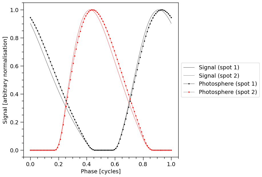
The pulse-profiles with markers are the signals incident on the telescope, before operating on them with the response model. The markers, linearly spaced in phase, denote the phase resolution.
The likelihood object calls the star.update method which in-turn calls the photosphere.embed method. The likelihood object then calls the photosphere.integrate method, passing the energies stored as the property signal.energies. We can do this manually if we wish to integrate signals but not calculate likelihoods. Here we sum over incident specific photon flux pulses as an approximation to integrating over energy. Note that we do not change the signal.signals traced
by the solid curves without markers.
[51]:
likelihood['cos_inclination'] = math.cos(1.0)

likelihood.externally_updated = True # declare safe to assume updates performed before call
xpsi.ParameterSubspace.__call__(likelihood) # no vector supplied
star.update()
photosphere.integrate(energies=signal.energies, threads=1)

XpsiPlot.plot_1d_pulse(signal=signal,
                       photosphere=photosphere,
                       photosphere_phases=signal.phases)
Notice the solid pulses without markers are unchanged from the plot a few cells above, and can be used to guide the eye to the effect of a change in Earth inclination.
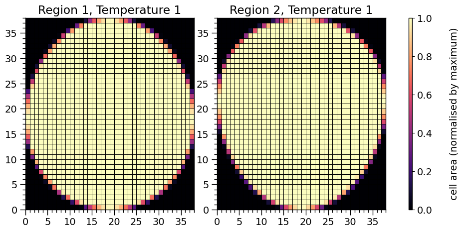
Below we print crude representations of the cell meshes spanning each hot region. The elements of a mesh cell-area array which are finite are not all identical: at the boundary of a hot region the proper area elements are smaller because of partial coverage by radiating material. The sum of all finite proper areas effectively equals the total proper area within a hot-region boundary.
[52]:
XpsiPlot.plot_meshes(regions=hot.objects)
Plotting the meshes for 2 regions, with 1 temperatures
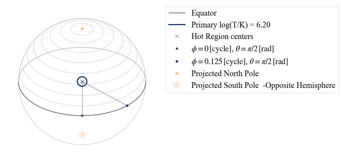
We can also use projection tool to visualize the geometry of the neutron star hot regions (see the separate documenation page for more information about the tool):
Note that the lowest colatitude row is at zero on the y-axis.
[53]:
from xpsi.utilities import ProjectionTool
[54]:
ProjectionTool.plot_projection_general((likelihood),"ST","I","NP")
YOU ARE USING 1 HOT SPOT MODEL
[54]:
<Axes: >
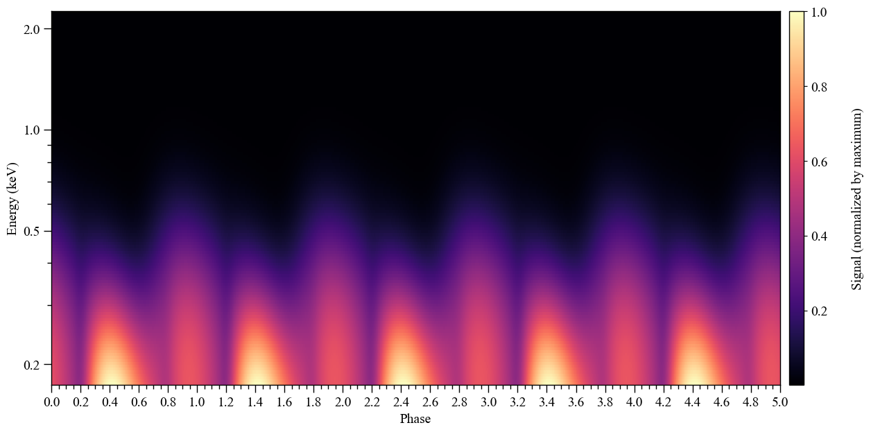
Let’s compute the incident specific flux signal normalised to the maximum and plot a pulse in two dimensions.
Note that if want to obtain the specific flux in units of photons/cm\(^{2}\)/s/keV instead, the output of photosphere.signal needs to be divided by distance squared, where distance is measured in meters.
Also note that we can interpolate the signal in phase as follows.
[55]:
from xpsi.tools import phase_interpolator

# Interpolation in phase with 500 phase bins
new_phases = np.linspace(0.0, 1, 500)

# Interpolating and summing spot1 (in photosphere.signal[0]) and spot2 (in photosphere.signal[1])
# with their respective signal phase shifts.

# SPOT 1 + SPOT 2
signal_photosphere = phase_interpolator(new_phases, signal.phases[0], photosphere.signal[0][0], signal.shifts[0]) +\
                     phase_interpolator(new_phases, signal.phases[0], photosphere.signal[1][0], signal.shifts[1])

XpsiPlot.plot_2d_pulse(signal_photosphere,
                       x=new_phases,
                       y=signal.energies,
                       rotations=5,
                       ylabel=r'Energy (keV)',
                       cbar_label=r'Signal (normalized by maximum)',
                       yticks=[0.2, 0.5, 1.0, 2.0],
                       normalized=True,
                      )
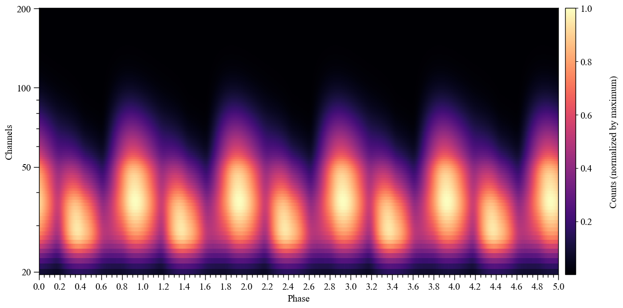
The count rate in each channel:
[56]:
new_phases = np.linspace(0.0, 1, 500)

# Interpolating and summing spot1 (in signal.signal[0]) and spot2 (in signal.signal[1])
# with their respective signal phase shifts.

# SPOT 1 + SPOT 2
signal_signal = phase_interpolator(new_phases, signal.phases[0], signal.signals[0], signal.shifts[0]) + \
                phase_interpolator(new_phases, signal.phases[0], signal.signals[1], signal.shifts[1])


XpsiPlot.plot_2d_pulse(signal_signal,
                       x=new_phases,
                       y=NICER.channels,
                       rotations=5,
                       ylabel=r'Channels',
                       cbar_label='Counts (normalized by maximum)',
                       yticks=[20,50,100,200],
                       normalized=True,
                      )
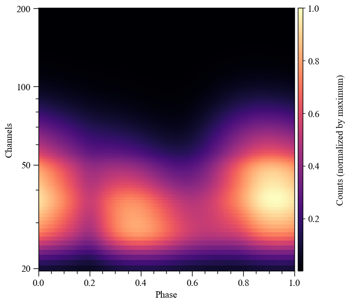
Now we increase the phase resolution, and plot a single rotational pulse:
[57]:
for obj in hot.objects:
    obj.set_phases(num_leaves = 1024)
# the current relationship between objects requires that we reinitialise
# if we wish to automatically communicate the updated settings between objects
p[3] = math.cos(1.0) # set inclination
_ = likelihood(p, reinitialise = True)
Note that reinitialisation also returned the following to default:
[58]:
likelihood.externally_updated
[58]:
False
[59]:
new_phases = np.linspace(0.0, 1, 500)

# SPOT 1 + SPOT 2
signal_signal = phase_interpolator(new_phases, signal.phases[0], signal.signals[0], signal.shifts[0]) + \
                phase_interpolator(new_phases, signal.phases[0], signal.signals[1], signal.shifts[1])

XpsiPlot.plot_2d_pulse(signal_signal,
                       x=new_phases,
                       y=NICER.channels,
                       rotations=1,
                       ylabel=r'Channels',
                       cbar_label='Counts (normalized by maximum)',
                       yticks=[20,50,100,200],
                       normalized=True,
                      )
Let’s iterate over a monotonically increasing set of values of the hot-region angular radius. Note that we use the keyword threads to directly instruct the low-level routines how many OpenMP threads to spawn to accelerate the computation. Usually the likelihood object instructs the low-level routines how many threads to spawn, based on it’s thread property:
[60]:
likelihood.threads
[60]:
1
Given that we are not currently using the likelihood object as a callback function passed to posterior sampling software (which parallelises efficiently using MPI), we can safely spawn additional OpenMP threads for signal integration; if likelihood evaluations are parallelised in an MPI environment on the other hand, one risks losing efficiency by spawning OpenMP threads for likelihood evaluation.
For objects that derive from ParameterSubspace we can get the current parameter vector in several ways:
[61]:
star()
[61]:
[1.4,
 12.5,
 0.2,
 0.5403023058681398,
 0.0,
 1.0,
 0.075,
 6.2,
 0.025,
 2.141592653589793,
 0.2]
[62]:
star() == star.vector # possible shortcut to save some characters
[62]:
True
The Likelihood subclass overrides the __call__ dunder, however, so we have to access it in the following ways:
[63]:
super(xpsi.Likelihood, likelihood).__call__() == likelihood.vector
[63]:
True
Note that we did not define any other parameters other than those associated with the star, and thus:
[64]:
len(likelihood) == len(star)
[64]:
True
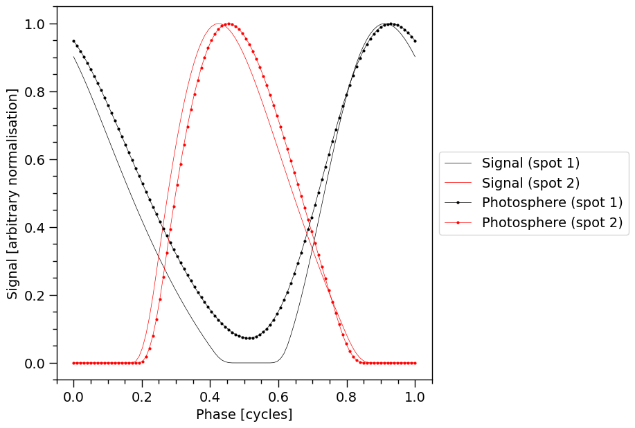
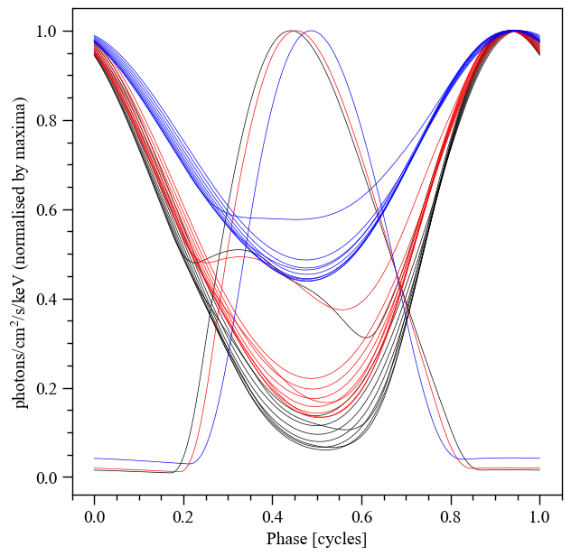
Finally, let’s play with some geometric parameters:
[65]:
fig = plt.figure(figsize=(7,7))
ax = fig.add_subplot(111)
ax.set_ylabel('photons/cm$^2$/s/keV (normalised by maxima)')
ax.set_xlabel('Phase [cycles]')

for obj in hot.objects:
    obj.set_phases(num_leaves = 256)

# let's play with the angular radius of the primary hot region
angular_radii = np.linspace(0.01, 1.0, 10)

likelihood.externally_updated = True

likelihood['cos_inclination'] = math.cos(1.25)

for angular_radius in angular_radii:
    likelihood['p__super_radius'] = angular_radius # play time
    star.update()
    photosphere.integrate(energies=signal.energies, threads=3)
    temp = np.sum(photosphere.signal[0][0] + photosphere.signal[1][0], axis=0)
    _ = ax.plot(hot.phases_in_cycles[0], temp/np.max(temp), 'k-', lw=0.5)

likelihood['cos_inclination'] = math.cos(1.0)

for angular_radius in angular_radii:
    likelihood['p__super_radius'] = angular_radius
    star.update()
    photosphere.integrate(energies=signal.energies, threads=3)
    temp = np.sum(photosphere.signal[0][0] + photosphere.signal[1][0], axis=0)
    _ = ax.plot(hot.phases_in_cycles[0], temp/np.max(temp), 'r-', lw=0.5)

likelihood['cos_inclination'] = math.cos(0.5)

for angular_radius in angular_radii:
    likelihood['p__super_radius'] = angular_radius
    star.update()
    photosphere.integrate(energies=signal.energies, threads=3)
    temp = np.sum(photosphere.signal[0][0] + photosphere.signal[1][0], axis=0)
    _ = ax.plot(hot.phases_in_cycles[0], temp/np.max(temp), 'b-', lw=0.5)

XpsiPlot.veneer((0.05,0.2), (0.05,0.2), ax)
Prior
Let us now construct a callable object representing a joint prior density distribution on the space \(\mathbb{R}^{d}\). We need to extend the base class to implement our distribution, which with respect to some parameters is separable, but for others it is uniform on a joint space, and compactly supported according to non-trivial constraint equations.
As an example gravitational mass and equatorial radius: a joint constraint is imposed to assign zero density to stars which are too compact: the polar radius, in units of the gravitational radius, of the rotationally deformed stellar 2-surface is too small.
Custom subclass
[66]:
from scipy.stats import truncnorm
[67]:
class CustomPrior(xpsi.Prior):
    """ A custom (joint) prior distribution.

    Source: Fictitious
    Model variant: ST-U
        Two single-temperature, simply-connected circular hot regions with
        unshared parameters.

    """

    __derived_names__ = ['compactness', 'phase_separation',]
    __draws_from_support__ = 3

    def __init__(self):
        """ Nothing to be done.

        A direct reference to the spacetime object could be put here
        for use in __call__:

        .. code-block::

            self.spacetime = ref

        Instead we get a reference to the spacetime object through the
        a reference to a likelihood object which encapsulates a
        reference to the spacetime object.

        """
        super(CustomPrior, self).__init__() # not strictly required if no hyperparameters

    def __call__(self, p = None):
        """ Evaluate distribution at ``p``.

        :param list p: Model parameter values.

        :returns: Logarithm of the distribution evaluated at ``p``.

        """
        temp = super(CustomPrior, self).__call__(p)
        if not np.isfinite(temp):
            return temp

        # based on contemporary EOS theory
        if not self.parameters['radius'] <= 16.0:
            return -np.inf

        ref = self.parameters.star.spacetime # shortcut

        # limit polar radius to try to exclude deflections >= \pi radians
        # due to oblateness this does not quite eliminate all configurations
        # with deflections >= \pi radians
        R_p = 1.0 + ref.epsilon * (-0.788 + 1.030 * ref.zeta)
        if R_p < 1.76 / ref.R_r_s:
            return -np.inf

        # polar radius at photon sphere for ~static star (static ambient spacetime)
        #if R_p < 1.5 / ref.R_r_s:
        #    return -np.inf

        mu = math.sqrt(-1.0 / (3.0 * ref.epsilon * (-0.788 + 1.030 * ref.zeta)))

        # 2-surface cross-section have a single maximum in |z|
        # i.e., an elliptical surface; minor effect on support, if any,
        # for high spin frequenies
        if mu < 1.0:
            return -np.inf

        ref = self.parameters # redefine shortcut

        # enforce order in hot region colatitude
        if ref['p__super_colatitude'] > ref['s__super_colatitude']:
            return -np.inf

        phi = (ref['p__phase_shift'] - 0.5 - ref['s__phase_shift']) * _2pi

        ang_sep = xpsi.HotRegion.psi(ref['s__super_colatitude'],
                                     phi,
                                     ref['p__super_colatitude'])

        # hot regions cannot overlap
        if ang_sep < ref['p__super_radius'] + ref['s__super_radius']:
            return -np.inf

        return 0.0

    def inverse_sample(self, hypercube=None):
        """ Draw sample uniformly from the distribution via inverse sampling. """

        to_cache = self.parameters.vector

        if hypercube is None:
            hypercube = np.random.rand(len(self))

        # the base method is useful, so to avoid writing that code again:
        _ = super(CustomPrior, self).inverse_sample(hypercube)

        ref = self.parameters # shortcut

        idx = ref.index('distance')
        ref['distance'] = truncnorm.ppf(hypercube[idx], -2.0, 7.0, loc=0.3, scale=0.1)

        # flat priors in cosine of hot region centre colatitudes (isotropy)
        # support modified by no-overlap rejection condition
        idx = ref.index('p__super_colatitude')
        a, b = ref.get_param('p__super_colatitude').bounds
        a = math.cos(a); b = math.cos(b)
        ref['p__super_colatitude'] = math.acos(b + (a - b) * hypercube[idx])

        idx = ref.index('s__super_colatitude')
        a, b = ref.get_param('s__super_colatitude').bounds
        a = math.cos(a); b = math.cos(b)
        ref['s__super_colatitude'] = math.acos(b + (a - b) * hypercube[idx])

        # restore proper cache
        for parameter, cache in zip(ref, to_cache):
            parameter.cached = cache

        # it is important that we return the desired vector because it is
        # automatically written to disk by MultiNest and only by MultiNest
        return self.parameters.vector

    def transform(self, p, **kwargs):
        """ A transformation for post-processing. """

        p = list(p) # copy

        # used ordered names and values
        ref = dict(zip(self.parameters.names, p))

        # compactness ratio M/R_eq
        p += [gravradius(ref['mass']) / ref['radius']]

        # phase separation between hot regions
        # first some temporary variables:
        if ref['p__phase_shift'] < 0.0:
            temp_p = ref['p__phase_shift'] + 1.0
        else:
            temp_p = ref['p__phase_shift']

        temp_s = 0.5 + ref['s__phase_shift']

        if temp_s > 1.0:
            temp_s = temp_s - 1.0

        # now append:
        if temp_s >= temp_p:
            p += [temp_s - temp_p]
        else:
            p += [1.0 - temp_p + temp_s]

        return p
[68]:
len(likelihood.vector)
[68]:
11
We can now construct and instantiate a callable prior object, pass it to the likelihood object, which stores a mutual reference to itself in prior. Note that if you have hyperparameters defined in the parameter subspace of prior, the prior needs to be passed upon instantiation of the likelihood object so that the hyperparameters get merged into the global parameter space; this is not demonstrated in this tutorial.
[69]:
prior = CustomPrior()
An empty subspace was created. This is normal behavior - no parameters were supplied.
[70]:
likelihood.prior = prior
[71]:
likelihood.merge(prior) # if there were hyperparameters, can merge them in
[72]:
likelihood.externally_updated = True # already set above, but for clarity
[73]:
prior() # a parameter vector is already stored
[73]:
0.0
We also defined a transform method:
[74]:
prior.transform(p)
[74]:
[1.4,
 12.5,
 0.2,
 0.5403023058681398,
 0.0,
 1.0,
 0.075,
 6.2,
 0.025,
 2.141592653589793,
 0.2,
 0.16538201343999998,
 0.525]
The penultimate entry is the compactness ratio M/R_eq, which should have a familar magnitude. The last entry is the phase separation in cycles.
The prior.inverse_sample() method is required by MultiNest to uniformly sample from the prior distribution and transform it into a posterior distribution. Let’s call the method, passing a vector of pseudorandom numbers drawn when each is drawn from a uniform distribution on the interval \([0,1)\):
[75]:
prior.inverse_sample()
[75]:
[2.9039112503473965,
 13.505293084374395,
 0.3452038792297925,
 0.22214114106361904,
 0.005637477633434362,
 2.2498632054765078,
 0.8025861833534218,
 3.408785205815536,
 0.2657943526445463,
 1.5656869839065086,
 0.5610250114920382]
In principle, inverse sampling from the prior can be used to initialise the ensemble of walkers evolved by emcee.
Density and support checking
Let’s draw samples from the prior and plot them:
[76]:
samps, _ = prior.draw(int(1e4))
Drawing samples from the joint prior...
Samples drawn.
Let’s first plot the \((M, R_{\rm eq})\) samples, with the Schwarzschild photon sphere and the radius prior.
[77]:
# Define the extra lines to plots together with the M-Req samples.
masses = np.linspace(1.0,3.0,100)
R_Schwarz = [3.0*gravradius(masses), masses]
R_Schwarz_label = r"Schwarzschild photon sphere $R_{eq} = 1.5 \times r_s(M)$"
R_prior = [2.0*1.76*gravradius(masses), masses]
R_prior_label = r"$R_{eq} = 1.76 \times r_s(M)$"
extra_plots = [R_Schwarz,R_prior,]
extra_labels = [R_Schwarz_label,R_prior_label,]


ax = XpsiPlot.plot_samps(samps,
                         x_idx=likelihood.index('radius'), # we can find the index for __getitem__ magic
                         y_idx=likelihood.index('mass'),
                         xlabel=likelihood.get_param('radius').symbol + ' [km]', # can use symbols like so
                         ylabel=r'$M$ [M$_{\odot}$]', # or manual entry
                         extras=extra_plots,
                         extras_label=extra_labels,
                        )
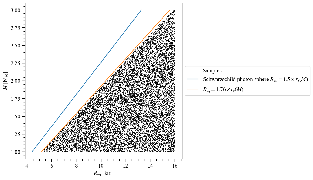
Note that the prior support is defined with a constraint that the polar radius \(R_{\rm p}(R_{\rm eq}, M, \Omega)\geq 1.76r_{s}(M)\), which is why there is a region devoid of samples between the prior support and the dashed line \(R_{\rm eq} = 1.76r_s(M)\). This condition is not necessary though because as of v0.6, X-PSI can include higher-order images, with the secondary and tertiary expected to be entirely sufficient in practice.
Let’s now plot the hot region (circular spot) colatitudes:
[78]:
# This diagonal show that we enforce colatitude order to distinguish hot regions as primary and secondary
diagonal = [np.array([0.0,math.pi]),np.array([0.0,math.pi])]
extra_plots = [diagonal, ]
extra_labels = ['diag']


ax = XpsiPlot.plot_samps(samps,
                         likelihood.index('p__super_colatitude'),
                         likelihood.index('s__super_colatitude'),
                         xlabel=r'$\Theta_{p}$ [radians]',
                         ylabel=r'$\Theta_{s}$ [radians]',
                         extras=extra_plots,
                         extras_label=extra_labels,
                        )
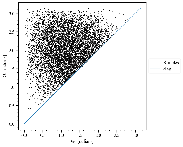
Note that the samples, marginalised over other region geometry parameters, are sparser when both hot regions approach the poles because we exclude overlapping configurations from the prior support. This is because the hot regions are by convention defined as disjoint, and cannot merge. If one wanted a more complex hot region, one would not invoke multiple hot regions that are permitted to overlap, but one would instead handle the extra complexity within the HotRegion class or a subclass.
Let’s plot the angular radii of the spots:
[79]:
ax = XpsiPlot.plot_samps(samps,
                         likelihood.index('p__super_radius'),
                         likelihood.index('s__super_radius'),
                         xlabel=r'$\zeta_{p}$ [radians]',
                         ylabel=r'$\zeta_{s}$ [radians]')
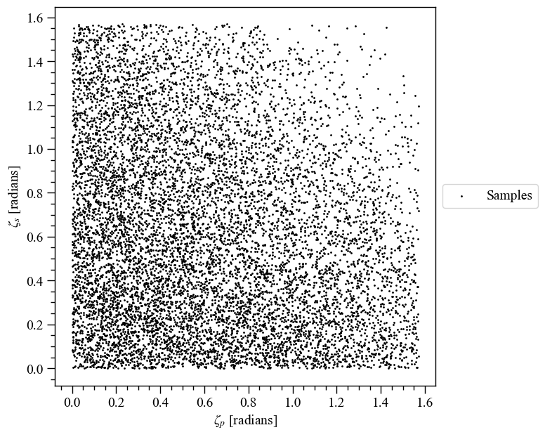
Note that the prior density is greater for hot regions that subtend smaller solid angles at the centre of the star, which also derives from the non-overlapping criterion for prior support.
Finally, let’s take a look at the phases:
[80]:
ax = XpsiPlot.plot_samps(samps,
                         likelihood.index('p__phase_shift'),
                         likelihood.index('s__phase_shift'),
                         xlabel=r'$\phi_{p}$ [cycles]',
                         ylabel=r'$\phi_{s}$ [cycles]')
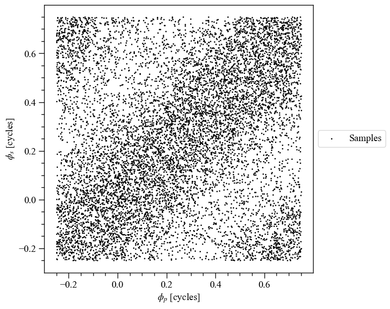
Note that again because the hot regions cannot overlap, rarefaction occurs in the vicinity of lines of minimal phase separation. Note that the boundaries are all periodic, so this pattern tesselates. Because we implemented a transformation in our CustomPrior subclass, we can actually draw the samples and transform them, which is useful in post-processing contexts. We defined the intervals [-0.25, 0.75] for the inverse sampling so that the posterior mode(s) will not be near a boundary.
The nested sampling algorithm can handle periodic boundaries by defining wrapped parameters; however, this can be trivially avoided altogether by rough inspection of the phases of the subpulses in the data, which we can see above are at around \(-0.1\) and \(0.4\) given the respective ground truth (injected) phases of \(\phi_{p}=0.0\) and \(\phi_{s}=0.025\).
Transformations for the purpose of likelihood evaluation must be handled in the inverse_sample method of an instance of the Prior class, but additional transformations that extend the parameter vector are written in the transform method.
If we wanted to transform automatically upon drawing the samples, thereby extending the parameter vectors passed to the __call__ method (so be careful with wrap-around indices when evaluating prior support conditions), we would do the following:
[81]:
samps_plus_transformed, _ = prior.draw(int(1e4), transform=True)
Drawing samples from the joint prior...
Samples drawn.
We defined a transformation from the hot region centre phases to the phase separation:
[82]:
ax = XpsiPlot.plot_samps(samps_plus_transformed,
                         likelihood.index('p__phase_shift'),
                         likelihood.prior.index('phase_separation'),
                         xlabel=r'$\phi_{p}$ [cycles]',
                         ylabel=r'$\Delta\phi$ [cycles]')
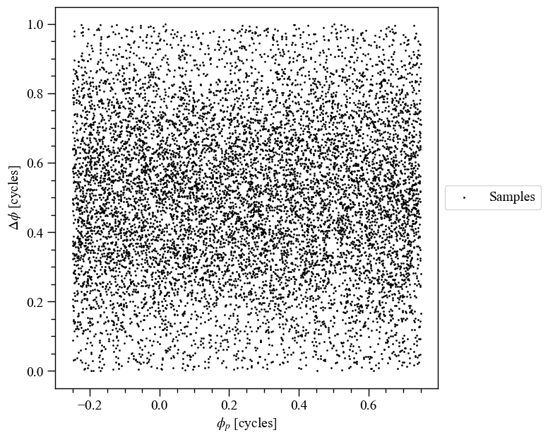
We can see the rarefaction occurs for \(\Delta\phi\sim0.0=1.0\).
The marginal one-dimensional prior distributions are overplotted, by the PostProcessing module, with the posterior distributions.
It is recommended to carefully inspect joint prior samples for pairs of parameters before commencing a sampling run, especially if there is a non-trivial constraint equation imposed on the prior support.
Sampling interface
We have constructed and instantiated both a callable likelihood object and a callable prior object. We could proceed, for example, to apply the open-source sampler PyMultiNest, emcee, or UltraNest to the joint posterior distribution proportional to the product of the (exponentiated) calls to the likelihood and prior objects.
MultiNest
We interface with the nested sampler MultiNest in a similar manner, by defining some runtime settings, and then passing those settings together with likelihood and prior objects to a wrapper from the Sample module. We will run the sampler for a specified number (10) of nested replacements (iterations). Note that the output below was actually generated with the temperature of the secondary hot region as a free parameter, resulting in an additional dimension to the model
above.
The environment variable LD_LIBRARY_PATH must be set before launching Jupyter as follows:
$ export LD_LIBRARY_PATH=<path/to/multinest>/lib
Get the parameters that are periodic or wrapped to inform MultiNest of boundary properties:
[83]:
wrapped_params = [0]*len(likelihood)
wrapped_params[likelihood.index('p__phase_shift')] = 1
wrapped_params[likelihood.index('s__phase_shift')] = 1
[84]:
os.system("mkdir -p run")

runtime_params = {'resume': False,
                  'importance_nested_sampling': False,
                  'multimodal': False,
                  'n_clustering_params': None,
                  'outputfiles_basename': './run/run', # make ./run directory manually
                  'n_iter_before_update': 5,
                  'n_live_points': 50, #100
                  'sampling_efficiency': 0.8,
                  'const_efficiency_mode': False,
                  'wrapped_params': wrapped_params,
                  'evidence_tolerance': 0.5,
                  'max_iter': 10, # 10000 # manual termination condition for short test
                  'verbose': True}

for h in hot.objects:
    h.set_phases(num_leaves = 100)

likelihood.threads = 3
likelihood.reinitialise()
likelihood.clear_cache()

# inform source code that parameter objects updated when inverse sampling
likelihood.externally_updated = True

p = [1.4,
     12.5,
     0.2,
     math.cos(1.25),
     0.0,
     1.0,
     0.075,
     6.2,
     0.025,
     math.pi - 1.0,
     0.2]

# let's require that checks pass before starting to sample
check_kwargs = dict(hypercube_points = None,
                    physical_points = p, # externally_updated preserved
                    loglikelihood_call_vals = [-2.6848565597e+04], # from above
                    rtol_loglike = 1.0e-6) # choose a tolerance

# note that mutual refs are already stored in the likelihood and prior
# objects to facilitate communication externally of the sampling process
xpsi.Sample.run_multinest(likelihood, prior, check_kwargs, **runtime_params)
Checking likelihood and prior evaluation before commencing sampling...
Not using ``allclose`` function from NumPy.
Using fallback implementation instead.
Checking closeness of likelihood arrays:
-2.6848565597e+04 | -2.6848565597e+04 .....
Closeness evaluated.
Log-likelihood value checks passed on root process.
Checks passed.
Commencing integration...
Estimating fractional hypervolume of the unit hypercube with finite prior density:
Requiring 1E+03 draws from the prior support for Monte Carlo estimation...
Drawing samples from the joint prior...
Samples drawn.
The support occupies an estimated 11.2% of the hypervolume within the unit hypercube...
Fractional hypervolume estimated.
Sampling efficiency set to: 7.1552.
 *****************************************************
 MultiNest v3.12
 Copyright Farhan Feroz & Mike Hobson
 Release Nov 2019

 no. of live points =   50
 dimensionality =   11
 *****************************************************
 Starting MultiNest
 generating live points
/tmp/ipykernel_40930/2552483892.py:52: DeprecationWarning: Conversion of an array with ndim > 0 to a scalar is deprecated, and will error in future. Ensure you extract a single element from your array before performing this operation. (Deprecated NumPy 1.25.)
  eval_marginal_likelihood(self._data.exposure_time,
 live points generated, starting sampling
  analysing data from ./run/run.txt
 ln(ev)=  -8.6284262997504847E+089 +/-                       NaN
 Total Likelihood Evaluations:           62
 Sampling finished. Exiting MultiNest
Integration completed.
The verbose output of the MultiNest program is by default directed to the host terminal session. Instead of trying to redirect that output to that of the above cell, we simply copy and paste the output from the terminal below. For the purpose of illustration, this output was for a 12-dimensional model variant (but using a longer test run).
*****************************************************
MultiNest v3.11
Copyright Farhan Feroz & Mike Hobson
Release Apr 2018

no. of live points =  100

dimensionality =   12
*****************************************************
Starting MultiNest
generating live points
 live points generated, starting sampling
Acceptance Rate:                        0.724638
Replacements:                                100
Total Samples:                               138
Nested Sampling ln(Z):            **************
Acceptance Rate:                        0.649351
Replacements:                                150
Total Samples:                               231
Nested Sampling ln(Z):            -116670.287917
Acceptance Rate:                        0.569801
Replacements:                                200
Total Samples:                               351
Nested Sampling ln(Z):            -115291.669431
Acceptance Rate:                        0.449640
Replacements:                                250
Total Samples:                               556
Nested Sampling ln(Z):            -108499.449911
Acceptance Rate:                        0.408719
Replacements:                                300
Total Samples:                               734
Nested Sampling ln(Z):             -95430.022790
Acceptance Rate:                        0.367261
Replacements:                                350
Total Samples:                               953
Nested Sampling ln(Z):             -77360.112633
Acceptance Rate:                        0.319744
Replacements:                                400
Total Samples:                              1251
Nested Sampling ln(Z):             -66119.380404
Acceptance Rate:                        0.263930
Replacements:                                450
Total Samples:                              1705
Nested Sampling ln(Z):             -57607.930990
Acceptance Rate:                        0.213675
Replacements:                                500
Total Samples:                              2340
Nested Sampling ln(Z):             -53505.956949
Acceptance Rate:                        0.173119
Replacements:                                550
Total Samples:                              3177
Nested Sampling ln(Z):             -50428.177797
Acceptance Rate:                        0.147893
Replacements:                                600
Total Samples:                              4057
Nested Sampling ln(Z):             -47108.755667
Acceptance Rate:                        0.132653
Replacements:                                650
Total Samples:                              4900
Nested Sampling ln(Z):             -43437.007007
Acceptance Rate:                        0.125381
Replacements:                                700
Total Samples:                              5583
Nested Sampling ln(Z):             -39888.092691
Acceptance Rate:                        0.113533
Replacements:                                750
Total Samples:                              6606
Nested Sampling ln(Z):             -36841.337131
Acceptance Rate:                        0.100251
Replacements:                                800
Total Samples:                              7980
Nested Sampling ln(Z):             -34450.919514
Acceptance Rate:                        0.088450
Replacements:                                850
Total Samples:                              9610
Nested Sampling ln(Z):             -32545.531967
Acceptance Rate:                        0.080121
Replacements:                                900
Total Samples:                             11233
Nested Sampling ln(Z):             -31270.147897
Acceptance Rate:                        0.069674
Replacements:                                950
Total Samples:                             13635
Nested Sampling ln(Z):             -30103.155016
Acceptance Rate:                        0.064201
Replacements:                               1000
Total Samples:                             15576
Nested Sampling ln(Z):             -29365.169148
Acceptance Rate:                        0.058427
Replacements:                               1050
Total Samples:                             17971
Nested Sampling ln(Z):             -28879.280235
 ln(ev)=  -28879.280235090871      +/-                       NaN
 Total Likelihood Evaluations:        17971
 Sampling finished. Exiting MultiNest
UltraNest
Another sampler that can be used as alternative to MultiNest is UltraNest. UltraNest contains many different sampling algorithms, but defaults to the nested sampling Monte Carlo MLFriends algorithm (Buchner, 2014; 2019). This is a type of region sampling similar to MultiNest, however, the way in which the shape and location of the ellipsoids is determined is different.
We interface with the sampler UltraNest is a similar manner as MultiNest: we define some runtime settings, and then pass those settings together with likelihood and prior objects to a wrapper from the Sample module. Note that the output below is generated with the temperature of the secondary hot region as a free parameter, similarly to the MultiNest example above.
In this example, we will run the sampler with a maximum of a 10 iterations. For a real inference problem, we don’t recommend this. See UltraNest’s FAQ and references therein for more information about choosing sampler settings.
To run UltraNest, we first define the parameters that are periodic or wrapped to inform UltraNest of boundary properties:
[85]:
wrapped_params = [False]*len(likelihood)
wrapped_params[likelihood.index('p__phase_shift')] = True
wrapped_params[likelihood.index('s__phase_shift')] = True
Next, we define the sampler_params which is a dictionary of the keyword arguments passed class Sample.UltranestSampler to initialise the sampler. UltraNest uses a reactive nested sampling algorithm, meaning it adapts the number of live points during the run. Therefore, we define a minimum (and maximum) number of live points instead of a fixed number.
Some useful keyword arguments that are not used in this example are:
log_dirto specify the directory where the output files are stored. As a default,log_dir='output', so the output will be stored in a folder calledoutputin the current directory. Unless otherwise specified, UltraNest will automatically create sub-directories called e.g.run1with incrementing numbers.resume=Truefor if you want to resume a run. As a default,resume=subfolderwhich creates a fresh sub-directory inlog_dir
[86]:
sampler_params = {'wrapped_params': wrapped_params}
We then also define the runtime_params which is a dictionary of the keyword arguments passed to the Sample.UltranestSampler to run the sampler. Next, we can start sampling:
[87]:
runtime_params = {'show_status':True, # show integration progress as a status line
                'min_num_live_points':400,
                'max_iters':10}

# let's sample!
xpsi.Sample.run_ultranest(likelihood,
                          prior,
                          sampler_params,
                          runtime_params)
Creating directory for new run output/run14
[ultranest] Sampling 400 live points from prior ...
/tmp/ipykernel_40930/2552483892.py:52: DeprecationWarning: Conversion of an array with ndim > 0 to a scalar is deprecated, and will error in future. Ensure you extract a single element from your array before performing this operation. (Deprecated NumPy 1.25.)
  eval_marginal_likelihood(self._data.exposure_time,
[ultranest] Explored until L=-1e+05   [-9.964e+89..-5.147e+89] | it/evals=0/401 eff=0.0000% N=400
[ultranest] Likelihood function evaluations: 410
[ultranest] Writing samples and results to disk ...
[ultranest] Writing samples and results to disk ... done
[ultranest]   logZ = -1.102e+05 +- 89.93
[ultranest] Effective samples strategy satisfied (ESS = 1.0, need >400)
[ultranest] Posterior uncertainty strategy wants to improve: -996424630216743409522701874586324452064573266569556541377719648531123882241807291728789504.00..-110133.81 (KL: 78.64+-105.44 nat, need <0.50 nat)
[ultranest] Evidency uncertainty strategy wants 398 minimum live points (dlogz from 78.69 to 183.61, need <0.5)
[ultranest]   logZ error budget: single: 0.12 bs:89.93 tail:0.69 total:89.93 required:<0.50
[ultranest] Widening from 1 to 800 live points before L=-1e+90...
[ultranest] parent value is -inf, so widening roots
[ultranest] Widening roots to 800 live points (have 400 already) ...
[ultranest] Sampling 400 live points from prior ...
/home/saltuomo/.conda/envs/xpsi_py3/lib/python3.12/site-packages/ultranest/integrator.py:1686: RuntimeWarning: invalid value encountered in divide
  p /= p.sum(axis=0).reshape((1, -1))
/tmp/ipykernel_40930/2552483892.py:52: DeprecationWarning: Conversion of an array with ndim > 0 to a scalar is deprecated, and will error in future. Ensure you extract a single element from your array before performing this operation. (Deprecated NumPy 1.25.)
  eval_marginal_likelihood(self._data.exposure_time,
[ultranest] Exploring (in particular: L=-inf..-110133.81) ...
[ultranest] Explored until L=-1e+05   [-inf..-1.101e+05] | it/evals=0/811 eff=0.0000% N=800
[ultranest] Likelihood function evaluations: 814
[ultranest] Writing samples and results to disk ...
[ultranest] Writing samples and results to disk ... done
[ultranest]   logZ = -1.096e+05 +- 327.1
[ultranest] Effective samples strategy satisfied (ESS = 1.0, need >400)
[ultranest] Posterior uncertainty strategy wants to improve: -998377734303308593861117534217346432286364882734806865666254240522771236219118721286799360.00..-109377.61 (KL: 216.10+-704.50 nat, need <0.50 nat)
[ultranest] Evidency uncertainty strategy wants 797 minimum live points (dlogz from 216.26 to 920.13, need <0.5)
[ultranest]   logZ error budget: single: 0.09 bs:327.14 tail:0.69 total:327.14 required:<0.50
[ultranest] Widening roots to 797 live points (have 800 already) ...
[ultranest] Exploring (in particular: L=-998377734303308593861117534217346432286364882734806865666254240522771236219118721286799360.00..-109377.61) ...
[ultranest] Explored until L=-1e+05
[ultranest] Likelihood function evaluations: 814
/home/saltuomo/.conda/envs/xpsi_py3/lib/python3.12/site-packages/ultranest/integrator.py:1686: RuntimeWarning: invalid value encountered in divide
  p /= p.sum(axis=0).reshape((1, -1))
[ultranest] Writing samples and results to disk ...
[ultranest] Writing samples and results to disk ... done
[ultranest] No changes made. Probably the strategy was to explore in the remainder, but it is irrelevant already; try decreasing frac_remain.
[ultranest] done iterating.

logZ = -109384.314 +- 0.851
  single instance: logZ = -109384.314 +- 0.000
  bootstrapped   : logZ = -109476.637 +- 0.493
  tail           : logZ = +- 0.693
insert order U test : converged: True correlation: inf iterations

    mass                : 1.000 │                ▇                      │1.960     1.410 +- 0.000
    radius              : 10.646│                   ▇                   │11.746    11.196 +- 0.000
    distance            : 0.100001809992010082│         ▇                             │0.775807257753374779    0.268871339355537420 +- 0.000000000000000056
    cos_inclination     : 0.34604879753366002│                                ▇      │0.99999899999999997    0.89604879753366029 +- 0.00000000000000022
    p__phase_shift      : 0.013 │                             ▇         │0.750     0.563 +- 0.000
    p__super_colatitude 1.29202359172447623 +- 0.00000000000000067
    p__super_radius     : 0.245 │                   ▇                   │1.345     0.795 +- 0.000
    p__super_temperature: 5.17792708948301694│                   ▇                   │6.27792708948301836    5.72792708948301854 +- 0.00000000000000089
    s__phase_shift      : 0.05178348433171726│                              ▇        │0.74999899999999997    0.60178348433171713 +- 0.00000000000000011
    s__super_colatitude 1.59784859362023091 +- 0.00000000000000022
    s__super_radius     : 0.32240235186611843│                   ▇                   │1.42240235186611863    0.87240235186611814 +- 0.00000000000000033
[87]:
<xpsi.UltranestSampler.UltranestSampler at 0x7a96f2a64590>
UltraNest also contains various step sampling algorithms which are generally better for high dimensional problems. In X-PSI, the slice sampling algorithm is implemented as step sampler. To use this, we need to set use_stepsampler=True and define a dictionary of keyword arguments passed to Sample.UltranestSampler to run the step sampler. The essential parameters:
nstepswhich define the number of accepted steps until the sample is considered independentgenerate_directionto specify the direction of the proposal function. The default isgenerate_mixture_random_direction, which is the one recommended in the UltraNest tutorials. This parameter is not shown in this example.
[88]:
stepsampler_params = {'nsteps':10}

xpsi.Sample.run_ultranest(likelihood,
                prior,
                sampler_params,
                runtime_params,
                use_stepsampler=True,
                stepsampler_params=stepsampler_params)
Creating directory for new run output/run15
[ultranest] Sampling 400 live points from prior ...
/tmp/ipykernel_40930/2552483892.py:52: DeprecationWarning: Conversion of an array with ndim > 0 to a scalar is deprecated, and will error in future. Ensure you extract a single element from your array before performing this operation. (Deprecated NumPy 1.25.)
  eval_marginal_likelihood(self._data.exposure_time,
[ultranest] Explored until L=-1e+05  e+05 [-9.952e+89..-4.536e+89] | it/evals=9/504 eff=8.6538% N=400
[ultranest] Likelihood function evaluations: 504
[ultranest] Writing samples and results to disk ...
[ultranest] Writing samples and results to disk ... done
[ultranest]   logZ = -1.101e+05 +- 190.6
[ultranest] Effective samples strategy satisfied (ESS = 1.0, need >400)
[ultranest] Posterior uncertainty strategy wants to improve: -995240421942427457844503901788709357661020286901403526555806306347807590479479125391179776.00..-109915.22 (KL: 145.05+-256.70 nat, need <0.50 nat)
[ultranest] Evidency uncertainty strategy wants 398 minimum live points (dlogz from 145.17 to 401.31, need <0.5)
[ultranest]   logZ error budget: single: 0.12 bs:190.64 tail:0.69 total:190.64 required:<0.50
[ultranest] Widening from 1 to 800 live points before L=-1e+90...
[ultranest] parent value is -inf, so widening roots
[ultranest] Widening roots to 800 live points (have 400 already) ...
[ultranest] Sampling 400 live points from prior ...
/home/saltuomo/.conda/envs/xpsi_py3/lib/python3.12/site-packages/ultranest/integrator.py:1686: RuntimeWarning: invalid value encountered in divide
  p /= p.sum(axis=0).reshape((1, -1))
/tmp/ipykernel_40930/2552483892.py:52: DeprecationWarning: Conversion of an array with ndim > 0 to a scalar is deprecated, and will error in future. Ensure you extract a single element from your array before performing this operation. (Deprecated NumPy 1.25.)
  eval_marginal_likelihood(self._data.exposure_time,
[ultranest] Exploring (in particular: L=-inf..-109915.22) ...
Z=-inf(0.00%) | Like=-1e+90..-1.1e+05 [-inf..-1.099e+05] | it/evals=0/915 eff=0.0000% N=800
/tmp/ipykernel_40930/2552483892.py:52: DeprecationWarning: Conversion of an array with ndim > 0 to a scalar is deprecated, and will error in future. Ensure you extract a single element from your array before performing this operation. (Deprecated NumPy 1.25.)
  eval_marginal_likelihood(self._data.exposure_time,
[ultranest] Explored until L=-1e+05  e+05 [-inf..-1.099e+05] | it/evals=8/955 eff=7.8431% N=800
[ultranest] Likelihood function evaluations: 965
[ultranest] Writing samples and results to disk ...
[ultranest] Writing samples and results to disk ... done
[ultranest]   logZ = -1.099e+05 +- 178.6
[ultranest] Effective samples strategy satisfied (ESS = 1.0, need >400)
[ultranest] Posterior uncertainty strategy wants to improve: -997977017685696158344953212720882826111069941253037761716280863829179433936443834592395264.00..-109819.97 (KL: 97.38+-391.74 nat, need <0.50 nat)
[ultranest] Evidency uncertainty strategy wants 795 minimum live points (dlogz from 97.53 to 488.67, need <0.5)
[ultranest]   logZ error budget: single: 0.09 bs:178.56 tail:0.69 total:178.56 required:<0.50
[ultranest] Widening roots to 795 live points (have 800 already) ...
[ultranest] Exploring (in particular: L=-997977017685696158344953212720882826111069941253037761716280863829179433936443834592395264.00..-109819.97) ...
[ultranest] Explored until L=-1e+05
[ultranest] Likelihood function evaluations: 965
/home/saltuomo/.conda/envs/xpsi_py3/lib/python3.12/site-packages/ultranest/integrator.py:1686: RuntimeWarning: invalid value encountered in divide
  p /= p.sum(axis=0).reshape((1, -1))
[ultranest] Writing samples and results to disk ...
[ultranest] Writing samples and results to disk ... done
[ultranest] No changes made. Probably the strategy was to explore in the remainder, but it is irrelevant already; try decreasing frac_remain.
[ultranest] done iterating.

logZ = -109826.673 +- 0.843
  single instance: logZ = -109826.673 +- 0.000
  bootstrapped   : logZ = -109921.051 +- 0.480
  tail           : logZ = +- 0.693
insert order U test : converged: True correlation: inf iterations
step sampler diagnostic: jump distance 0.88 (should be >1), far enough fraction: 43.75% : very fishy. Double nsteps and see if fraction and lnZ change)

    mass                : 1.24229367601560181│                   ▇                   │2.34229367601560146    1.79229367601560230 +- 0.00000000000000067
    radius              : 10.4475378402528776│                   ▇                   │11.5475378402528790    10.9975378402528765 +- 0.0000000000000018
    distance            : 0.100001809992010082│      ▇                                │0.755156946046478206    0.205156946046478134 +- 0.000000000000000028
    cos_inclination     : 0.16483652459422510│                         ▇             │0.99999899999999997    0.71483652459422520 +- 0.00000000000000011
    p__phase_shift      : -0.250│      ▇                                │0.410     -0.140 +- 0.000
    p__super_colatitude 1.31188026935313418 +- 0.00000000000000044
    p__super_radius     : 0.000 │   ▇                                   │0.596     0.046 +- 0.000
    p__super_temperature: 5.37863908084137954│                   ▇                   │6.47863908084138096    5.92863908084137936 +- 0.00000000000000089
    s__phase_shift      : -0.250│       ▇                               │0.439     -0.111 +- 0.000
    s__super_colatitude 2.067 +- 0.000
    s__super_radius     : 0.000 │                ▇                      │0.970     0.420 +- 0.000

step sampler diagnostic: jump distance 0.88 (should be >1), far enough fraction: 43.75% : very fishy. Double nsteps and see if fraction and lnZ change)
[88]:
<xpsi.UltranestSampler.UltranestSampler at 0x7a96f0406d50>
In addition to UltraNest’s standard output files, a .txt file with the default name weighted_post_ultranest_xpsi is created when the inference finished. This file can be used for post-processing within X-PSI as usual.
Ensemble MCMC
To prove that the objects constructed above can be fed to the emcee sampler, let’s run a number of iterations using a single Python process. We will initialise the ensemble by drawing from a multivariate Gaussian with mean vector equal to the ground truth (injected) vector.
[89]:
std = [1.0,
         0.05,
         1.0,
         0.01,
         0.05,
         0.0025,
         0.01,
         0.05,
         0.05,
         0.01,
         0.01]

runtime_params = {'resume': False,
                  'root_dir': './',
                  'nwalkers': 50,
                  'nsteps': 10,
                  'walker_dist_moments': zip(p, std)} #  if resume then ``None``

for h in hot.objects:
    h.set_phases(num_leaves = 100) # revert to original phase resolution above

likelihood.threads = 3
likelihood.reinitialise() # because we played with the object above

# Use MPI=False for testing purposes
backend = xpsi.Sample.run_emcee(likelihood, prior,
                                MPI=False, **runtime_params)
Warning: a ``samples.h5`` file exists in ``./``.
Attempting to move ``samples.h5`` to a subdirectory of ``./``.
File archived in subdirectory ``./old_samples``.

Commencing posterior sampling.
/tmp/ipykernel_40930/2552483892.py:52: DeprecationWarning: Conversion of an array with ndim > 0 to a scalar is deprecated, and will error in future. Ensure you extract a single element from your array before performing this operation. (Deprecated NumPy 1.25.)
  eval_marginal_likelihood(self._data.exposure_time,
100%|██████████████████████████████████████████████████████████████████████████████████████| 10/10 [03:09<00:00, 18.90s/it]
Sampling complete.
[90]:
# clean up the docs/source directory
#!rm samples.h5; rm -r old_samples
Note that we could also try initialising the ensemble by inverse sampling the joint prior distribution.
Let’s quickly plot the evolution of the ensemble Markov chains to prove that the sampling process commenced and is behaving in a somewhat reasonable manner:
[91]:
try:
    backend
except NameError:
    import emcee
    backend = emcee.backends.HDFBackend('samples.h5')

chain = backend.get_chain()

# These chains plotted were generated using
# v0.2 so the labels here are in a different
# order. The model also had two free
# temperature parameters instead of just one.
# Also, inclination was the parameter, not
# cos(inclination), and the prior was flat
# in inclination, not cos(inclination).
labels = [r'$D$',
          r'$M$',
          r'$R_{\rm eq}$',
          r'$\cos(i)$',
          r'$\phi_{p}$',
          r'$\Theta_{p}$',
          r'$\zeta_{p}$',
          r'$T_{p}$',
          r'$\phi_{s}$'
          r'$\Theta_{s}$',
          r'$\zeta_{s}$']

fig = plt.figure(figsize=(8,32))

gs = gridspec.GridSpec(12, 1, hspace=0.15)

for i in range(len(labels)):
    ax = plt.subplot(gs[i,0])
    ax.set_ylabel(labels[i])
    for j in range(50):
        plt.plot(chain[:,j,i], 'k-', lw=0.5, alpha=0.5)
    if i < 11:
        ax.tick_params(axis='x', labelbottom=False)
        plt.setp(ax.get_yticklabels()[0], visible=False)
        plt.setp(ax.get_yticklabels()[-1], visible=False)
    else: ax.set_xlabel('Steps')
    XpsiPlot.veneer((250, 1000), None, ax)
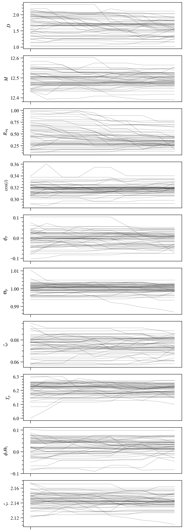
The chains rendered in the documentation were run on a desktop machine in about a day of wall-time. It is visually discernable that the ensemble distribution has not yet evolved to a stationary state: a rigourous application of ensemble MCMC would cover convergence criteria, auto-correlation, and examination of sensitivity to initial conditions and the transition kernel. In fact, based on the analysis with nested sampling on path xpsi/examples/default_background, we know that the posterior
mode in the vicinity of the above ensemble is rather non-linear in the space being sampled, so ensemble MCMC may require many steps in order to argue for convergence.
Synthesis
In this notebook thus far we have not generated sythetic data. However, we did condition on synthetic data. Below we outline how that data was generated. More information about synthetic data generation can be found in the “Instrument Synergy” and “Synthesise Data” tutorial notebooks.
Background
The background radiation field incident on the model instrument for the purpose of generating synthetic data was a time-invariant powerlaw spectrum, and was transformed into a count-rate in each output channel using the response matrix for synthetic data generation. We would reproduce this background here by writing a custom subclass as follows.
[92]:
class CustomBackground(xpsi.Background):
    """ The background injected to generate synthetic data. """

    def __init__(self, bounds=None, value=None):

        # first the parameters that are fundemental to this class
        doc = """
        Powerlaw spectral index.
        """
        index = xpsi.Parameter('powerlaw_index',
                                strict_bounds = (-3.0, -1.01),
                                bounds = bounds,
                                doc = doc,
                                symbol = r'$\Gamma$',
                                value = value)

        super(CustomBackground, self).__init__(index)

    def __call__(self, energy_edges, phases):
        """ Evaluate the incident background field. """

        G = self['powerlaw_index']

        temp = np.zeros((energy_edges.shape[0] - 1, phases.shape[0]))

        temp[:,0] = (energy_edges[1:]**(G + 1.0) - energy_edges[:-1]**(G + 1.0)) / (G + 1.0)

        for i in range(phases.shape[0]):
            temp[:,i] = temp[:,0]

        self._incident_background = temp
Note that the analytic background is integrated over energy intervals, as required by a Signal instance, which would then straightforwardly apply the model instrument response to the background.
We can now construct and instantiate a background object. The base clase xpsi.Background is inherited from the ParameterSubspace ABC. We therefore need to specify the number of background parameters, and define the hard bounds on those parameters; in this case we have only a single parameter, the powerlaw index.
We would then instantiate as follows:
[93]:
background = CustomBackground(bounds=(None, None)) # use strict bounds, but do not fix/derive
Creating parameter:
    > Named "powerlaw_index" with bounds [-3.000e+00, -1.010e+00].
    > Powerlaw spectral index.
Data format
We are also in need of a simpler data object.
[94]:
class SynthesiseData(xpsi.Data):
    """ Custom data container to enable synthesis. """

    def __init__(self, channels, phases, first, last):

        self.channels = channels
        self._phases = phases

        try:
            self._first = int(first)
            self._last = int(last)
        except TypeError:
            raise TypeError('The first and last channels must be integers.')
        if self._first >= self._last:
            raise ValueError('The first channel number must be lower than the '
                             'the last channel number.')
Instantiate:
[95]:
_data = SynthesiseData(np.arange(20,201), np.linspace(0.0, 1.0, 33), 0, 180)
Setting channels for event data...
Channels set.
Custom method
We are in need of a synthesise method, which in this implementation wraps an extension module. Let’s check what the extension module offers:
When creating synthetic data, we can fix the random seed for noise by providing it as an input parameter called ‘gsl_seed’. If no input is provided, the seed is based on the clock time.
Add unbound methods:
Instantiate, and reconfigure the likelihood object:
[96]:
signal = CustomSignal(data = _data,
                        instrument = NICER,
                        background = background,
                        interstellar = None,
                        min_channel=20,
                        max_channel=200,
                        prefix='NICER')

for h in hot.objects:
    h.set_phases(num_leaves = 100)

likelihood = xpsi.Likelihood(star = star, signals = signal, threads=1)
Trimming event data...
WARNING : There is no counts in data object. This is normal if you are trying to synthesise data.Otherwise something is very wrong and do not continue
Trimming instrument response...
Setting channels for loaded instrument response (sub)matrix...
Channels set.
Instrument response trimmed.
Creating parameter:
    > Named "phase_shift" with fixed value 0.000e+00.
    > The phase shift for the signal, a periodic parameter [cycles].
Warning: No data... can synthesise data but cannot evaluate a likelihood function.
Synthesise
[97]:
p = [1.4,
     12.5,
     0.2,
     math.cos(1.25),
     0.0,
     1.0,
     0.075,
     6.2,
     0.025,
     math.pi - 1.0,
     0.2,
     -2.0]

NICER_kwargs = dict(expected_source_counts=2.0e6,
                    expected_background_counts=2.0e6,
                    name='new_synthetic',
                    directory='../../examples/examples_fast/Data')

likelihood.synthesise(p, force=True, NICER=NICER_kwargs)
Using background from signal._background.
[98]:
XpsiPlot.plot_2d_pulse(pulse=np.loadtxt('../../examples/examples_fast/Data/new_synthetic_realisation.dat', dtype=np.double),
                       x=_data.phases,
                       y=_data.channels,
                       rotations=1,
                       ylabel='Channel',
                       cbar_label='Counts',)
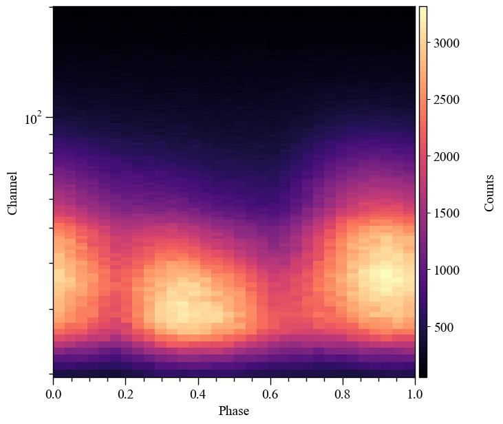
Some differences may exist between the newly created synthetic data and the synthetic data found in the GitHub examples (especially at the lowest energy channels), because these were created with different interpolators (periodic Steffen spline and Akima periodic).
[99]:
diff = data.counts - np.loadtxt('../../examples/examples_fast/Data/new_synthetic_realisation.dat', dtype=np.double)
(diff != 0.0).any()
[99]:
True
Summary
In this notebook we constructed a model including a likelihood and prior objects. We also looked at the sampling interface, and concluded by synthesising the pre-prepared data set that was loaded at the beginning of the notebook.