Instrument synergy
The purpose of this notebook is to prototype support for multiple instruments operating on the same signal incident at Earth. The instruments may have different wavebands and the data may or may not be phase resolved for each instrument.
Some extra data files not available on the GitHub repository are needed to run this tutorial. They can be found in the Zenodo and should be placed in the directory examples/examples_modeling_tutorial/model_data/ of your local xpsi directory. These are the required files:
nicer_v1.01_arf.txtnicer_v1.01_rmf_matrix.txtnicer_v1.01_rmf_energymap.txt
[1]:
%matplotlib inline

import os
import numpy as np
import math
import time

from matplotlib import pyplot as plt
from matplotlib import rcParams
from matplotlib.ticker import MultipleLocator, AutoLocator, AutoMinorLocator
from matplotlib import gridspec
from matplotlib import cm
rcParams['text.usetex'] = False
rcParams['font.size'] = 14.0

import xpsi

from xpsi.global_imports import _c, _G, _dpr, gravradius, _csq, _km, _2pi
from xpsi.utilities import PlottingLibrary as XpsiPlot
/=============================================\
| X-PSI: X-ray Pulse Simulation and Inference |
|---------------------------------------------|
|                Version: 3.3.0               |
|---------------------------------------------|
|      https://xpsi-group.github.io/xpsi      |
\=============================================/

Imported emcee version: 3.1.6
Imported PyMultiNest.
Imported UltraNest.
Imported GetDist version: 1.5.3
Imported nestcheck version: 0.2.1
[2]:
class Telescope(object):
    pass
[3]:
NICER = Telescope()
XMM = Telescope() # fabricated toy that we'll just pretend is XMM as a placeholder!
Likelihood
Let us load a synthetic data set that we generated in advance, and know the fictitious exposure time for.
[4]:
obs_settings = dict(counts=np.loadtxt('../../examples/examples_modeling_tutorial/model_data/example_synthetic_realisation.dat', dtype=np.double),
                    channels=np.arange(20, 201),
                    phases=np.linspace(0.0, 1.0, 33),
                    first=0,last=180,
                    exposure_time=984307.6661)

NICER.data = xpsi.Data(**obs_settings)
Setting channels for event data...
Channels set.
[5]:
obs_settings = dict(counts=np.loadtxt('../../examples/examples_modeling_tutorial/model_data/XMM_realisation.dat', dtype=np.double).reshape(-1,1),
                    channels=np.arange(20, 201),
                    phases=np.array([0.0, 1.0]),
                    first=0,last=180,
                    exposure_time=1818434.247359)

XMM.data = xpsi.Data(**obs_settings)
Setting channels for event data...
Channels set.
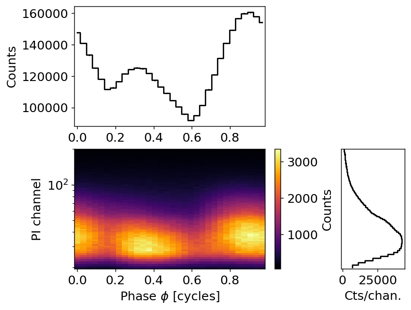
Now for the data:
[6]:
fig, axs = NICER.data.plot(dpi=130, num_rot=1)
[7]:
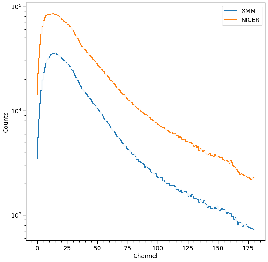
print(f"XMM data is a spectrum. The array shape is : {np.shape(XMM.data.counts)}")
print(f"NICER data is a pulse profile. They array shape is : {np.shape(NICER.data.counts)}")

data_to_plot = [XMM.data.counts,
                np.sum(NICER.data.counts, axis=1)]  # Summing the NICER pulse profile over phase-bin to make spectrum
label_to_plot = ['XMM', 'NICER']

XpsiPlot.plot_spectrum(all_data=data_to_plot,
                       all_labels=label_to_plot)
XMM data is a spectrum. The array shape is : (181, 1)
NICER data is a pulse profile. They array shape is : (181, 32)
Instrument
We require a model instrument object to transform incident specific flux signals into a form which enters directly in the sampling distribution of the data.
[8]:
class CustomInstrument(xpsi.Instrument):
    """ A model of the NICER telescope response. """

    def __call__(self, signal, *args):
        """ Overwrite base just to show it is possible.

        We loaded only a submatrix of the total instrument response
        matrix into memory, so here we can simplify the method in the
        base class.

        """

        matrix = self.construct_matrix()

        self._folded_signal = np.dot(matrix, signal)

        return self._folded_signal

    @classmethod
    def from_response_files(cls, ARF, RMF, channel_edges, max_input, min_input=0,
                            translate_edges=None, scaling=None, inst_name=None):
        """ Constructor which converts response files into :class:`numpy.ndarray`s.
        :param str ARF: Path to ARF which is compatible with
                                :func:`numpy.loadtxt`.
        :param str RMF: Path to RMF which is compatible with
                                :func:`numpy.loadtxt`.
        :param str channel_edges: Path to edges which is compatible with
                                  :func:`numpy.loadtxt`.
        :param float translate_edges: Optional translation of the energy edges (in keV).
        :param float scaling: Optional Scaling to scale the ARF.

        """

        if min_input != 0:
            min_input = int(min_input)

        max_input = int(max_input)

        try:
            ARF = np.loadtxt(ARF, dtype=np.double, skiprows=3)
            RMF = np.loadtxt(RMF, dtype=np.double)
            channel_edges = np.loadtxt(channel_edges, dtype=np.double, skiprows=3)[:,1:]
        except:
            print('A file could not be loaded.')
            raise

        if scaling is not None:
            ARF[:,3] *= scaling

        matrix = np.ascontiguousarray(RMF[min_input:max_input,20:201].T, dtype=np.double)

        edges = np.zeros(ARF[min_input:max_input,3].shape[0]+1, dtype=np.double)

        edges[0] = ARF[min_input,1]; edges[1:] = ARF[min_input:max_input,2]

        for i in range(matrix.shape[0]):
            matrix[i,:] *= ARF[min_input:max_input,3]

        channels = np.arange(20, 201)

        if translate_edges is not None:
            edges += translate_edges

        Inst = cls(matrix, edges, channels, channel_edges[20:202,-2])
        Inst.name = inst_name
        return Inst
Let’s construct an instance of the first instrument called NICER. This is made from RMF and ARF in ASCII (text) file format, but a new loader from FITS file is available (see “Modelling” tutorial).
[9]:
NICER.instrument = CustomInstrument.from_response_files(ARF = '../../examples/examples_modeling_tutorial/model_data/nicer_v1.01_arf.txt',
                                         RMF = '../../examples/examples_modeling_tutorial/model_data/nicer_v1.01_rmf_matrix.txt',
                                         channel_edges = '../../examples/examples_modeling_tutorial/model_data/nicer_v1.01_rmf_energymap.txt',
                                         max_input = 500,
                                         min_input = 0,
                                         inst_name='NICER XTI')
Setting channels for loaded instrument response (sub)matrix...
Channels set.
An empty subspace was created. This is normal behavior - no parameters were supplied.
For the second instrument, called XMM, we use the some response files (those of NICER) with two additional arbitrary modifications (for the sake of the example):
add a
scaling=0.5which reduces the sensitivity by half (seeCustomInstrumentclass above).add a
translate_edges=0.1which shifts the sensitivity matrix by 0.1 keV.
[10]:
XMM.instrument = CustomInstrument.from_response_files(ARF = '../../examples/examples_modeling_tutorial/model_data/nicer_v1.01_arf.txt',
                                       RMF = '../../examples/examples_modeling_tutorial/model_data/nicer_v1.01_rmf_matrix.txt',
                                       channel_edges = '../../examples/examples_modeling_tutorial/model_data/nicer_v1.01_rmf_energymap.txt',
                                       max_input = 500,
                                       min_input = 0,
                                       translate_edges = 0.1,
                                       scaling = 0.5,
                                       inst_name='XMM')
Setting channels for loaded instrument response (sub)matrix...
Channels set.
An empty subspace was created. This is normal behavior - no parameters were supplied.
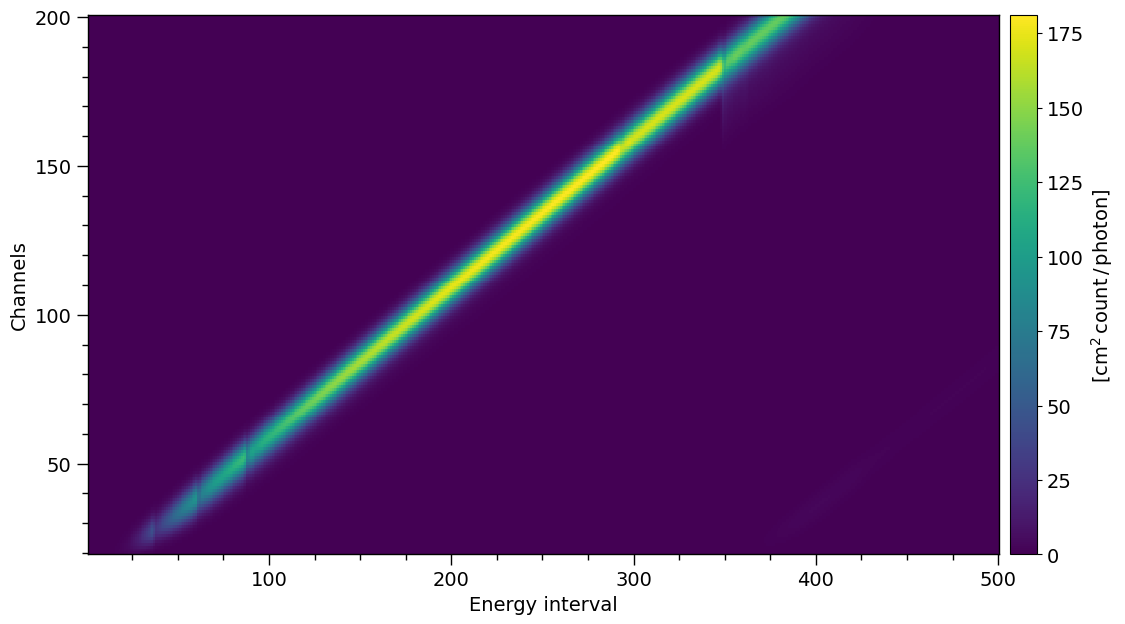
The NICER v1.01 response matrix:
[11]:
energy_inputs = np.arange(1,len( NICER.instrument.energy_edges)+1)-0.5
channels = NICER.instrument.channel_edges * 100 - 0.5

rmf_plot = XpsiPlot.plot_rmf(matrix=NICER.instrument.matrix,
                             x=energy_inputs,
                             y=channels,
                             xlabel='Energy interval',
                             ylabel='Channels'
                            )

XpsiPlot.veneer((25, 100), (10, 50), rmf_plot)
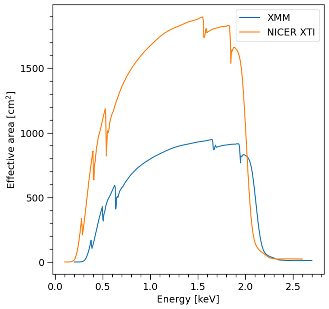
Summed over channel subset \([20,200]\):
[12]:
arfplot = XpsiPlot.plot_arf([XMM.instrument, NICER.instrument])
XpsiPlot.veneer((0.1, 0.5), (100, 500), arfplot)
Pile-up
Some X-ray detectors (e.g., CCD) may suffer from pile-up, which happens when more than one photon is incident on the same pixel of the detectors within one read-out time (or frame time). CCD can take several seconds (e.g., up to 3.2 sec for Chandra ACIS-I) to completely read all pixels. During this time, bright X-ray sources may cause two or more X-ray photons to fall on the same pixels. The detectors will therefore account for a single event with energy equal to the sum of the energies of the incident photons during that readout time. This distorts the X-ray spectrum to higher energies. For a given readout time, the brighter the X-ray source, the stronger the effects of pile-up.
Pile-up can be mitigated by reducing the CCD read-out time with a faster mode, for ex., by restricting the readout area to a sub-portion of the CCD. For Chandra, the readout time can be reduced to 0.4 sec by selecting 1/8 of the CCD to be used.
Nonetheless, if the pile-up effects are still presents (e.g., 1 or 2 % of photons are piled-up), a correction to the spectral model might be necessary to limit biases in the inferred spectral parameters. To do so, a statistical accounting of piled-up photons can account for these effects. Mathematically, this is means that pile-up correction function (see Davis 2001 ) needs to be convolved first to ARF * spectral_model and
the result to RMF. To perform this efficiently for inferrence in X-PSI, this product of convolutions is done in Fourier space.
In practice, the InstrumentPileup class will do all this in X-PSI. It works as the Instrument class, but it includes two extra parameter:
grade_migration, which gives the probability that an event with two or more photons was not rejected, i.e., that it corresponds to a piled-up event.psf_fraction, which corresponds to the fraction of the telescope point spread fonction in which pile-up is consider (fixed by default at 95%, and can be fitted).
So grade_migration is the only parameter of the pile-up model that really needs to be fitted. Two other (fixed) parameters, frame_time and frac_expo, are read directly from the header of the data file (this requires to load the data from a FITS file).
Signal
[13]:
from xpsi.likelihoods.default_background_marginalisation import eval_marginal_likelihood
from xpsi.likelihoods.default_background_marginalisation import precomputation

class CustomSignal(xpsi.Signal):
    """ A custom calculation of the logarithm of the likelihood.
    We extend the :class:`xpsi.Signal.Signal` class to make it callable.
    We overwrite the body of the __call__ method. The docstring for the
    abstract method is copied.
    """

    def __init__(self, workspace_intervals = 1000, epsabs = 0, epsrel = 1.0e-8,
                 epsilon = 1.0e-3, sigmas = 10.0, support = None, *args, **kwargs):
        """ Perform precomputation. """

        super(CustomSignal, self).__init__(*args, **kwargs)

        try:
            self._precomp = precomputation(self._data.counts.astype(np.int32))
        except AttributeError:
            print('Warning: No data... can synthesise data but cannot evaluate a '
                  'likelihood function.')
        else:
            self._workspace_intervals = workspace_intervals
            self._epsabs = epsabs
            self._epsrel = epsrel
            self._epsilon = epsilon
            self._sigmas = sigmas
            if support is not None:
                self._support = support
            else:
                self._support = -1.0 * np.ones((self._data.counts.shape[0],2))
                self._support[:,0] = 0.0

    @property
    def support(self):
        return self._support

    @support.setter
    def support(self, obj):
        self._support = obj

    def __call__(self, **kwargs):
        self.loglikelihood, self.expected_counts, self.background_signal, self.background_given_support = \
                eval_marginal_likelihood(self._data.exposure_time,
                                          self._data.phases,
                                          self._data.counts,
                                          self._signals,
                                          self._phases,
                                          self._shifts,
                                          self._precomp,
                                          self._support,
                                          self._workspace_intervals,
                                          self._epsabs,
                                          self._epsrel,
                                          self._epsilon,
                                          self._sigmas,
                                          kwargs.get('llzero'))
Note that if we need an additional overall phase shift parameter for additional instruments whose recorded data are phase resolved, then it could be passed to the subclass above for the signal associated with a given telescope.
[14]:
NICER.signal = CustomSignal(data = NICER.data,
                              instrument = NICER.instrument,
                              background = None,
                              interstellar = None,
                              workspace_intervals = 1000,
                              epsrel = 1.0e-8,
                              epsilon = 1.0e-3,
                              sigmas = 10.0)
Creating parameter:
    > Named "phase_shift" with fixed value 0.000e+00.
    > The phase shift for the signal, a periodic parameter [cycles].
[15]:
XMM.signal = CustomSignal(data = XMM.data,
                               instrument = XMM.instrument,
                               background = None,
                               interstellar = None,
                               support = None,
                               workspace_intervals = 1000,
                               epsrel = 1.0e-8,
                               epsilon = 1.0e-3,
                               sigmas = 10.0)
Creating parameter:
    > Named "phase_shift" with fixed value 0.000e+00.
    > The phase shift for the signal, a periodic parameter [cycles].
Star
[16]:
bounds = dict(distance = (None, None),                   # (Earth) distance
                mass = (None, None),                     # mass
                radius = (None, None),                   # equatorial radius
                cos_inclination = (None, None))          # (Earth) inclination to rotation axis

values = dict(frequency=300.0 )                          # spin frequency

spacetime = xpsi.Spacetime(bounds=bounds, values=values)
Creating parameter:
    > Named "frequency" with fixed value 3.000e+02.
    > Spin frequency [Hz].
Creating parameter:
    > Named "mass" with bounds [1.000e-03, 3.000e+00].
    > Gravitational mass [solar masses].
Creating parameter:
    > Named "radius" with bounds [1.000e+00, 2.000e+01].
    > Coordinate equatorial radius [km].
Creating parameter:
    > Named "distance" with bounds [1.000e-02, 3.000e+01].
    > Earth distance [kpc].
Creating parameter:
    > Named "cos_inclination" with bounds [-1.000e+00, 1.000e+00].
    > Cosine of Earth inclination to rotation axis.
[17]:
bounds = dict(super_colatitude = (None, None),
              super_radius = (None, None),
              phase_shift = (-0.5, 0.5),
              super_temperature = (None, None))

# a simple circular, simply-connected spot
primary = xpsi.HotRegion(bounds=bounds,
                            values={}, # no initial values and no derived/fixed
                            symmetry=True,
                            omit=False,
                            cede=False,
                            concentric=False,
                            sqrt_num_cells=32,
                            min_sqrt_num_cells=10,
                            max_sqrt_num_cells=64,
                            num_leaves=100,
                            num_rays=200,
                            prefix='p') # unique prefix needed because >1 instance
Creating parameter:
    > Named "super_colatitude" with bounds [0.000e+00, 3.142e+00].
    > The colatitude of the centre of the superseding region [radians].
Creating parameter:
    > Named "super_radius" with bounds [0.000e+00, 1.571e+00].
    > The angular radius of the (circular) superseding region [radians].
Creating parameter:
    > Named "phase_shift" with bounds [-5.000e-01, 5.000e-01].
    > The phase of the hot region, a periodic parameter [cycles].
Creating parameter:
    > Named "super_temperature" with bounds [3.000e+00, 7.600e+00].
    > log10(superseding region effective temperature [K]).
[18]:
class derive(xpsi.Derive):
    def __init__(self):
        """
        We can pass a reference to the primary here instead
        and store it as an attribute if there is risk of
        the global variable changing.

        This callable can for this simple case also be
        achieved merely with a function instead of a magic
        method associated with a class.
        """
        pass

    def __call__(self, boundto, caller = None):
        # one way to get the required reference
        global primary # unnecessary, but for clarity
        return primary['super_temperature'] - 0.2

bounds['super_temperature'] = None # declare fixed/derived variable

secondary = xpsi.HotRegion(bounds=bounds, # can otherwise use same bounds
                              values={'super_temperature': derive()}, # create a callable value
                              symmetry=True,
                              omit=False,
                              cede=False,
                              concentric=False,
                              sqrt_num_cells=32,
                              min_sqrt_num_cells=10,
                              max_sqrt_num_cells=100,
                              num_leaves=100,
                              num_rays=200,
                              is_antiphased=True,
                              prefix='s') # unique prefix needed because >1 instance
Creating parameter:
    > Named "super_colatitude" with bounds [0.000e+00, 3.142e+00].
    > The colatitude of the centre of the superseding region [radians].
Creating parameter:
    > Named "super_radius" with bounds [0.000e+00, 1.571e+00].
    > The angular radius of the (circular) superseding region [radians].
Creating parameter:
    > Named "phase_shift" with bounds [-5.000e-01, 5.000e-01].
    > The phase of the hot region, a periodic parameter [cycles].
Creating parameter:
    > Named "super_temperature" that is derived from ulterior variables.
    > log10(superseding region effective temperature [K]).
[19]:
from xpsi import HotRegions

hot = HotRegions((primary, secondary))
[20]:
class CustomPhotosphere(xpsi.Photosphere):
    """ Implement method for imaging."""

    def _global_variables(self):

        return np.array([self['p__super_colatitude'],
                          self['p__phase_shift'] * _2pi,
                          self['p__super_radius'],
                          self['p__super_temperature'],
                          self['s__super_colatitude'],
                          (self['s__phase_shift'] + 0.5) * _2pi,
                          self['s__super_radius'],
                          self.hot.objects[1]['s__super_temperature']])
[21]:
photosphere = CustomPhotosphere(hot = hot, elsewhere = None,
                                values=dict(mode_frequency = spacetime['frequency']))
Creating parameter:
    > Named "mode_frequency" with fixed value 3.000e+02.
    > Coordinate frequency of the mode of radiative asymmetry in the
photosphere that is assumed to generate the pulsed signal [Hz].
[22]:
star = xpsi.Star(spacetime = spacetime, photospheres = photosphere)
[23]:
likelihood = xpsi.Likelihood(star = star, signals = [NICER.signal, XMM.signal],
                             threads = 1, externally_updated = False)
The instrument wavebands exhibit a high degree of overlap. The energies at which we compute incident specific flux signals are based on the union of wavebands, distributed logarithmically:
[24]:
fig = plt.figure(figsize=(8,8))
plt.plot(XMM.signal.energies, 'kx')
ax = plt.gca()
ax.set_xlabel('Index')
_ = ax.set_ylabel('Energy [keV]')
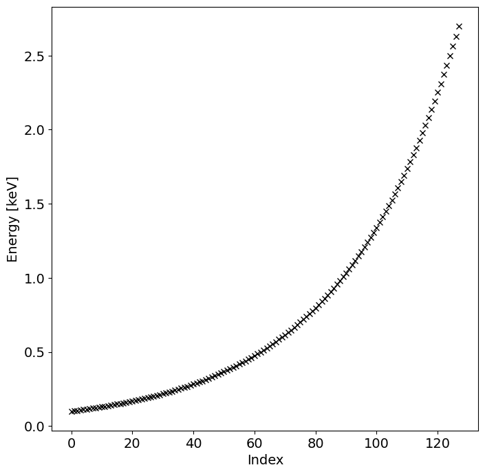
This is a simple, non-adaptive protocol to ensure that signals are not computed at very nearby energies for multiple telescopes, resulting in overhead.
Let’s call the likelihood object with the true model parameter values that we injected to generate the synthetic data rendered above, omitting background parameters:
[25]:
p = [1.4,
     12.5,
     0.2,
     math.cos(1.25),
     0.0,
     1.0,
     0.075,
     6.2,
     0.025,
     math.pi - 1.0,
     0.2]

t = time.time()
ll = likelihood(p, force=True) # force if you want to clear parameter value caches

print('ll = %.8f; time = %.3f' % (ll, time.time() - t))
ll = -30055.76414850; time = 0.948
[26]:
NICER.signal.loglikelihood # check NICER ll ~ -26713.602 ?
[26]:
-27446.923112789216
[27]:
XMM.signal.loglikelihood # check XMM ll ~ -2608.841 ?
[27]:
-2608.84103571022
Let’s fabricate some rough prior information as the constrained support of the background parameters for XMM:
[28]:
support = np.zeros((181, 2))
support[:,0] = XMM.signal.background_signal - 5.0 * np.sqrt(XMM.signal.background_signal)
support[:,1] = XMM.signal.background_signal + 5.0 * np.sqrt(XMM.signal.background_signal)
support /= XMM.data.exposure_time
[29]:
XMM.signal.support = support
[30]:
ll = likelihood(p, force=True)
Let’s confirm that the XMM background-marginalised likelihood did indeed change:
[31]:
XMM.signal.loglikelihood
[31]:
-2610.1216095310615
The background-marginalised likelihood function has the following form. Subscripts N denote NICER, whilst subscripts X denote XMM.
The term \(p(\{\mathbb{E}[b_{\rm X}]\} \,|\, \{b_{\rm X}\})\) truncates the integral over XMM channel-by-channel background count rate variables to an interval \([a,b]\) in each channel, where \(a,b\in\mathbb{R}^{+}\). This is the joint prior support of the variables \(\{\mathbb{E}[b_{\rm X}]\}\) rendered in the spectral plot below. The form of the prior density \(p(\{\mathbb{E}[b_{\rm X}]\} \,|\, \{b_{\rm X}\})\) is flat on this interval for each channel. This is a simplifying approximation to the probability of the background data \(\{b_{\rm X}\}\) given the variables \(\{\mathbb{E}[b_{\rm X}]\}\).
[32]:
support_data = [support[:,0]*XMM.data.exposure_time, support[:,1]*XMM.data.exposure_time ]

data_to_plot = [XMM.signal.background_signal,
                XMM.signal.expected_counts,
                XMM.data.counts,
                support_data
               ]
label_to_plot = ['MCL background',
                 'MCL counts given support',
                'XMM data',
                 'support'
                ]

XpsiPlot.plot_spectrum(data_to_plot, all_labels=label_to_plot, thickness=[2,5,2,14])
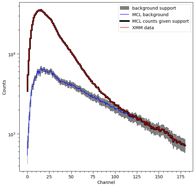
The spectrum labelled MCL counts given support means the expected signal from the pulsar, plus the background count vector that maximises the conditional likelihood function given that pulsar signal, subject to the background vector existing in the prior support. The spectrum labelled MCL background, on the other hand, is the background vector that maximises the conditional likelihood function, but not subject to the prior support.
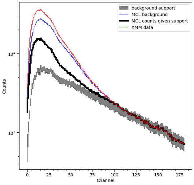
[33]:
likelihood['p__super_temperature'] = 6.1
[34]:
likelihood.externally_updated = True
[35]:
likelihood()
[35]:
-388650.02566585346
[36]:
XMM.signal.loglikelihood
[36]:
-321117.06212714006
[37]:
support_data = [support[:,0]*XMM.data.exposure_time, support[:,1]*XMM.data.exposure_time ]

data_to_plot = [XMM.signal.background_signal,
                XMM.signal.expected_counts,
                XMM.data.counts,
                support_data
               ]
label_to_plot = ['MCL background',
                 'MCL counts given support',
                 'XMM data',
                 'support'
                ]

XpsiPlot.plot_spectrum(data_to_plot, all_labels=label_to_plot, thickness=[2,5,2,14])
Synthesis
In this notebook thus far we have not generated sythetic data. However, we did condition on synthetic data. Below we outline how that data was generated.
Background
The background radiation field incident on the model instrument for the purpose of generating synthetic data was a time-invariant powerlaw spectrum, and was transformed into a count-rate in each output channel using the response matrix for synthetic data generation. We would reproduce this background here by writing a custom subclass as follows.
[38]:
class CustomBackground(xpsi.Background):
    """ The background injected to generate synthetic data. """

    def __init__(self, bounds=None, value=None):

        # first the parameters that are fundemental to this class
        doc = """
        Powerlaw spectral index.
        """
        index = xpsi.Parameter('powerlaw_index',
                                strict_bounds = (-3.0, -1.01),
                                bounds = bounds,
                                doc = doc,
                                symbol = r'$\Gamma$',
                                value = value,
                                permit_prepend = False) # because to be shared by multiple objects

        super(CustomBackground, self).__init__(index)

    def __call__(self, energy_edges, phases):
        """ Evaluate the incident background field. """

        G = self['powerlaw_index']

        temp = np.zeros((energy_edges.shape[0] - 1, phases.shape[0]))

        temp[:,0] = (energy_edges[1:]**(G + 1.0) - energy_edges[:-1]**(G + 1.0)) / (G + 1.0)

        for i in range(phases.shape[0]):
            temp[:,i] = temp[:,0]

        self._incident_background = temp
[39]:
background = CustomBackground(bounds=(None, None)) # use strict bounds, but do not fix/derive
Creating parameter:
    > Named "powerlaw_index" with bounds [-3.000e+00, -1.010e+00].
    > Powerlaw spectral index.
We will use this same background signal, albeit with different normalisations, for both telescopes. This is simply to generate finite background contributions.
Data format
We are also in need of a simpler data object.
[40]:
class SynthesiseData(xpsi.Data):
    """ Custom data container to enable synthesis. """

    def __init__(self, channels, phases, first, last):
        self.channels = channels
        self._phases = phases

        try:
            self._first = int(first)
            self._last = int(last)
        except TypeError:
            raise TypeError('The first and last channels must be integers.')
        if self._first >= self._last:
            raise ValueError('The first channel number must be lower than the '
                             'the last channel number.')
Instantiate:
[41]:
NICER.synth = SynthesiseData(np.arange(20,201), np.linspace(0.0, 1.0, 33), 0, 180)
Setting channels for event data...
Channels set.
[42]:
XMM.synth = SynthesiseData(np.arange(20,201), np.array([0.0,1.0]), 0, 180)
Setting channels for event data...
Channels set.
Custom method
[43]:
from xpsi.tools.synthesise import synthesise_given_total_count_number as _synthesise
We now need to instantiate, and reconfigure the likelihood object:
[44]:
NICER.signal = CustomSignal(data = NICER.synth,
                              instrument = NICER.instrument,
                              background = background,
                              interstellar = None,
                              workspace_intervals = 1000,
                              epsrel = 1.0e-8,
                              epsilon = 1.0e-3,
                              sigmas = 10.0,
                              prefix='NICER')

XMM.signal = CustomSignal(data = XMM.synth,
                          instrument = XMM.instrument,
                          background = background,
                          interstellar = None,
                          workspace_intervals = 1000,
                          epsrel = 1.0e-8,
                          epsilon = 1.0e-3,
                          sigmas = 10.0,
                          prefix='XMM')

for h in hot.objects:
    h.set_phases(num_leaves = 100)

likelihood = xpsi.Likelihood(star = star, signals = [NICER.signal, XMM.signal], threads=1)
Creating parameter:
    > Named "phase_shift" with fixed value 0.000e+00.
    > The phase shift for the signal, a periodic parameter [cycles].
Warning: No data... can synthesise data but cannot evaluate a likelihood function.
Creating parameter:
    > Named "phase_shift" with fixed value 0.000e+00.
    > The phase shift for the signal, a periodic parameter [cycles].
Warning: No data... can synthesise data but cannot evaluate a likelihood function.
Synthesise
We proceed to synthesise.
[45]:
likelihood
[45]:
Free parameters
---------------
mass: Gravitational mass [solar masses].
radius: Coordinate equatorial radius [km].
distance: Earth distance [kpc].
cos_inclination: Cosine of Earth inclination to rotation axis.
p__phase_shift: The phase of the hot region, a periodic parameter [cycles].
p__super_colatitude: The colatitude of the centre of the superseding region [radians].
p__super_radius: The angular radius of the (circular) superseding region [radians].
p__super_temperature: log10(superseding region effective temperature [K]).
s__phase_shift: The phase of the hot region, a periodic parameter [cycles].
s__super_colatitude: The colatitude of the centre of the superseding region [radians].
s__super_radius: The angular radius of the (circular) superseding region [radians].
powerlaw_index: Powerlaw spectral index.
[46]:
p = [1.4,
     12.5,
     0.2,
     math.cos(1.25),
     0.0,
     1.0,
     0.075,
     6.2,
     0.025,
     math.pi - 1.0,
     0.2,
     -2.0]

NICER_kwargs = dict(expected_source_counts = 2.0e6,
                    expected_background_counts = 2.0e6,
                    name = 'new_NICER',
                    directory = '../../examples/examples_fast/Data')

XMM_kwargs = dict(expected_source_counts = 1.0e6,
                  expected_background_counts = 5.0e5,
                  name = 'new_XMM',
                  directory = '../../examples/examples_fast/Data')

likelihood.synthesise(p,
                      force = True,
                      NICER = NICER_kwargs,
                      XMM = XMM_kwargs)
Using background from signal._background.
Using background from signal._background.
Notice that the normalisations, with units photons/s/cm^2/keV, are different because we require so many background counts. This detail is unimportant for this notebook, wherein we simply want some finite background contributions.
[47]:
XpsiPlot.plot_2d_pulse(pulse=np.loadtxt('../../examples/examples_fast/Data/new_NICER_realisation.dat', dtype=np.double),
                       x=NICER.data.phases,
                       y=NICER.data.channels,
                       rotations=1,
                       ylabel='Channel',
                       cbar_label='Counts',)
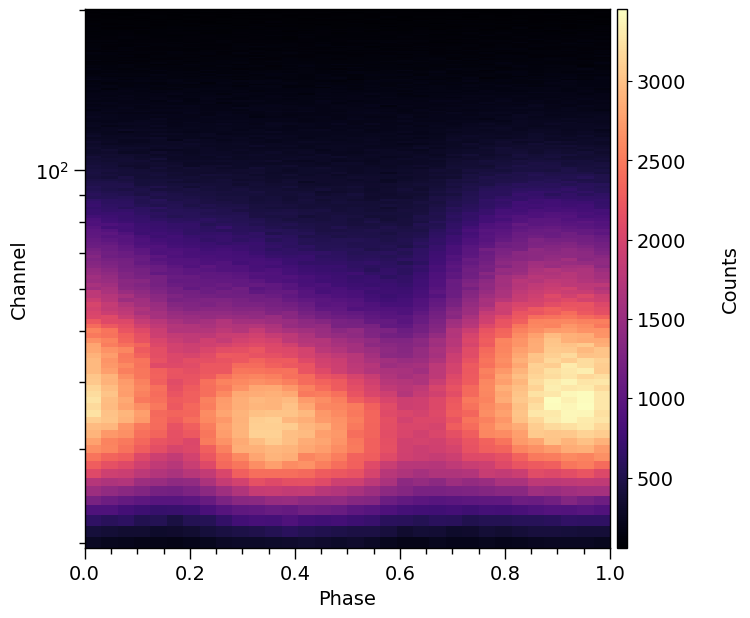
Check we have generated the same count numbers, given the same seed and resolution settings:
[48]:
diff = XMM.data.counts - np.loadtxt('../../examples/examples_fast/Data/new_XMM_realisation.dat', dtype=np.double).reshape(-1,1)
(diff != 0.0).any()
[48]:
True
[49]:
diff = NICER.data.counts - np.loadtxt('../../examples/examples_fast/Data/new_NICER_realisation.dat', dtype=np.double)
(diff != 0.0).any()
[49]:
True
Some differences may exist between the newly created synthetic data and the synthetic data found in the GitHub examples (especially at the lowest energy channels). This is because the example data were produced using significantly newer NICER response files.
Saving synthetic data to FITS file (event or PHA)
[50]:
NICER_kwargs = dict(expected_source_counts = 2.0e6,
                    expected_background_counts = 2.0e6,
                    format='FITS',
                    instrument_name = 'PN_MOS',
                    name = 'new_NICER',
                    directory = '../../examples/examples_fast/Data')

XMM_kwargs = dict(expected_source_counts = 1.0e6,
                  expected_background_counts = 5.0e5,
                  format='FITS',
                  instrument_name = 'XMM_MOS',
                  name = 'new_XMM',
                  directory = '../../examples/examples_fast/Data')

likelihood.synthesise(p,
                      force = True,
                      NICER = NICER_kwargs,
                      XMM = XMM_kwargs,
                      )
Using background from signal._background.
Using background from signal._background.
[51]:
!ls ../../examples/examples_fast/Data/*evt ../../examples/examples_fast/Data/*pha
../../examples/examples_fast/Data/new_NICER_bkg.evt
../../examples/examples_fast/Data/new_NICER_bkg_realisation.evt
../../examples/examples_fast/Data/new_NICER.evt
../../examples/examples_fast/Data/new_NICER_realisation.evt
../../examples/examples_fast/Data/new_synthetic_bkg.evt
../../examples/examples_fast/Data/new_synthetic_bkg_realisation.evt
../../examples/examples_fast/Data/new_synthetic.evt
../../examples/examples_fast/Data/new_synthetic_realisation.evt
../../examples/examples_fast/Data/new_XMM_bkg.evt
../../examples/examples_fast/Data/new_XMM_bkg.pha
../../examples/examples_fast/Data/new_XMM_bkg_realisation.evt
../../examples/examples_fast/Data/new_XMM_bkg_realisation.pha
../../examples/examples_fast/Data/new_XMM.pha
../../examples/examples_fast/Data/new_XMM_realisation.pha