Global surface emission
Let’s explore simulation of signals generated by surface radiation fields that globally span the star.
We will also perform weak internal cross-checking of integrators that are algorithmically distinct in their discretisation of the computational domain. For instance, regular discretisation can be performed: (i) on a spacelike 2-surface embedded in an ambient Schwarzschild spacetime, yielding a moving mesh (between temporal hyperslices of the spacetime foliation) that tracks modes of radiative asymmetry; (ii) on a spacelike 2-surface embedded in an ambient Schwarzschild spacetime, yielding a static mesh that does not move (between temporal hyperslices of the spacetime foliation) but plasma and modes of radiative asymmetry to flow through it; and (iii) on a distant image-plane through which radiation flows normally en route to some effectively asymptotic receiver.
To run the end part of this tutorial, starting from “Custom (phase-dependent)”, you’ll have to switch the contents of the ``xpsi/surface_radiation_field/local_variables.pyx`` extension and re-install X-PSI, as instructed below, in order to change the mapping from global variables to local variables. However, the beginning part of the tutorial, “Default (phase-invariant)”, should be run using the default extension.
[1]:
%matplotlib inline

from __future__ import print_function, division

import os
import numpy as np
import math

from matplotlib import pyplot as plt
from matplotlib import rcParams
from matplotlib.ticker import MultipleLocator, AutoLocator, AutoMinorLocator
from matplotlib import gridspec
from matplotlib import cm

from IPython.display import Image

import xpsi
from xpsi import Parameter

from xpsi.global_imports import _c, _G, _dpr, gravradius, _csq, _km, _2pi
/=============================================\
| X-PSI: X-ray Pulse Simulation and Inference |
|---------------------------------------------|
|                Version: 3.3.0               |
|---------------------------------------------|
|      https://xpsi-group.github.io/xpsi      |
\=============================================/

Imported emcee version: 3.1.6
Imported PyMultiNest.
Imported UltraNest.
Imported GetDist version: 1.5.3
Imported nestcheck version: 0.2.1
[2]:
from xpsi.tools import phase_interpolator

def plot_2D_pulse(z, x, shift, y, ylabel,
                  num_rotations=5.0, res=5000, normalise=True,
                  error=False,
                  cm=cm.viridis, vmin=None, vmax=None, label=None):
    """ Helper function to plot a phase-energy pulse.

    :param array-like z:
        Either one, or a pair, of *ndarray[m,n]* objects representing the signal at
        *n* phases and *m* values of an energy variable. A pair is required if
        the fractional difference is to be plotted.

    :param ndarray[n] x: Phases the signal is resolved at.

    :param float shift: Phase shift to apply.

    :param ndarray[m] y: Energy values the signal is resolved at.

    """

    fig = plt.figure(figsize = (12,6))

    gs = gridspec.GridSpec(1, 2, width_ratios=[50,1], wspace=0.025)
    ax = plt.subplot(gs[0])
    ax_cb = plt.subplot(gs[1])

    new_phases = np.linspace(0.0, num_rotations, res)

    if error:
        interpolated = phase_interpolator(new_phases,
                                      x,
                                      np.ascontiguousarray(z[0]), shift)

        interpolated /= phase_interpolator(new_phases,
                                      x,
                                      np.ascontiguousarray(z[1]), shift)

        interpolated -= 1.0
        interpolated *= 100.0

        vmax = np.max(np.abs(interpolated))
        vmin = -vmax

    else:
        interpolated = phase_interpolator(new_phases,
                                      x,
                                      np.ascontiguousarray(z), shift)

        if normalise:
            interpolated /= np.max(interpolated)

        if vmin is None:
            vmin = np.min(interpolated)

        if vmax is None:
            vmax = np.max(interpolated)

    profile = ax.pcolormesh(new_phases,
                             y,
                             interpolated,
                             cmap = cm,
                             vmin = vmin,
                             vmax = vmax,
                             linewidth = 0,
                             rasterized = True)

    profile.set_edgecolor('face')

    ax.set_xlim([0.0, num_rotations])
    ax.set_yscale('log')
    ax.set_ylabel(ylabel)
    ax.set_xlabel(r'Phase')
    veneer((0.1, 0.5), (None,None), ax)

    cb = plt.colorbar(profile,
                      cax = ax_cb,
                      ticks = AutoLocator())

    cb.set_label(label=label or r'Signal (normalised by maximum)', labelpad=25)
    cb.solids.set_edgecolor('face')

    cb.outline.set_linewidth(1.0)

rcParams['text.usetex'] = False
rcParams['font.size'] = 18.0

def veneer(x, y, axes, lw=1.0, length=8):
    """ Make the plots a little more aesthetically pleasing. """
    if x is not None:
        if x[1] is not None:
            axes.xaxis.set_major_locator(MultipleLocator(x[1]))
        if x[0] is not None:
            axes.xaxis.set_minor_locator(MultipleLocator(x[0]))
    else:
        axes.xaxis.set_major_locator(AutoLocator())
        axes.xaxis.set_minor_locator(AutoMinorLocator())

    if y is not None:
        if y[1] is not None:
            axes.yaxis.set_major_locator(MultipleLocator(y[1]))
        if y[0] is not None:
            axes.yaxis.set_minor_locator(MultipleLocator(y[0]))
    else:
        axes.yaxis.set_major_locator(AutoLocator())
        axes.yaxis.set_minor_locator(AutoMinorLocator())

    axes.tick_params(which='major', colors='black', length=length, width=lw)
    axes.tick_params(which='minor', colors='black', length=int(length/2), width=lw)
    plt.setp(axes.spines.values(), linewidth=lw, color='black')
First we need to do some setup of the ambient spacetime and the surface embedded in it that the photosphere exists on.
[3]:
bounds = dict(distance = (0.1, 1.0),                     # (Earth) distance
                mass = (1.0, 3.0),                       # mass
                radius = (3.0 * gravradius(1.0), 16.0),  # equatorial radius
                cos_inclination = (0.0, 1.0))      # (Earth) inclination to rotation axis

spacetime = xpsi.Spacetime(bounds=bounds, values=dict(frequency=600.0))
Creating parameter:
    > Named "frequency" with fixed value 6.000e+02.
    > Spin frequency [Hz].
Creating parameter:
    > Named "mass" with bounds [1.000e+00, 3.000e+00].
    > Gravitational mass [solar masses].
Creating parameter:
    > Named "radius" with bounds [4.430e+00, 1.600e+01].
    > Coordinate equatorial radius [km].
Creating parameter:
    > Named "distance" with bounds [1.000e-01, 1.000e+00].
    > Earth distance [kpc].
Creating parameter:
    > Named "cos_inclination" with bounds [0.000e+00, 1.000e+00].
    > Cosine of Earth inclination to rotation axis.
Default (phase-invariant)
First we invoke a globally uniform temperature field. There is no azimuthal dependence, meaning that the signal generated by the star is time-invariant. We are in need of an object that embeds a globally discretised surface into the ambient spacetime and exposes methods for integration over solid angle on our sky.
[4]:
bounds = dict(temperature = (None, None))

everywhere = xpsi.Everywhere(time_invariant=True,
                             bounds=bounds,
                             values={}, # no fixed/derived variables
                             sqrt_num_cells=512,
                             num_rays=512,
                             num_leaves=512,
                             num_phases=100) # specify leaves if time-dependent
Warning : with time_invariant=True, num_leaves and num_phases are automatically set to 1
Creating parameter:
    > Named "temperature" with bounds [3.000e+00, 7.600e+00].
    > log10(effective temperature [K] everywhere).
Creating parameter:
    > Named "phase_shift" with fixed value 0.000e+00.
We are free to subclass Everywhere and implement custom functionality beyond the simple default above. The argument specifying the number of rays has the familiar meaning. The argument for the number of cells is now used to discretise the surface in azimuth and colatitude with respect to the stellar rotation axis, as was the case for the Elsewhere module. The new argument time_invariant declares
whether or not the surface radiation field is dependent on azimuth; if it is independent of azimuth, a faster integrator is called.
Now we need an instance of Photosphere that we can feed our everywhere object to.
[5]:
photosphere = xpsi.Photosphere(hot = None, elsewhere = None, everywhere = everywhere,
                               values=dict(mode_frequency = spacetime['frequency']))
Creating parameter:
    > Named "mode_frequency" with fixed value 6.000e+02.
    > Coordinate frequency of the mode of radiative asymmetry in the
photosphere that is assumed to generate the pulsed signal [Hz].
[6]:
star = xpsi.Star(spacetime = spacetime, photospheres = photosphere)
Let’s check the vector of parameter values in the Star instance and the other objects it encapsulates references to.
[7]:
star
[7]:
Free parameters
---------------
mass: Gravitational mass [solar masses].
radius: Coordinate equatorial radius [km].
distance: Earth distance [kpc].
cos_inclination: Cosine of Earth inclination to rotation axis.
temperature: log10(effective temperature [K] everywhere).
[8]:
def set_defaults():
    global star # for clarity
    # (Earth) distance
    star['distance'] = 0.33
    # gravitational mass
    star['mass'] = 2.0
    # coordinate equatorial radius
    star['radius'] = 12.0
    # (Earth) inclination to rotation axis
    star['cos_inclination'] = math.cos(1.0)
    # isotropic blackbody temperature
    star['temperature'] = 5.7

set_defaults()
We assign parameter values and update the star as follows:
[9]:
star['temperature'] = 6.0

star.update()
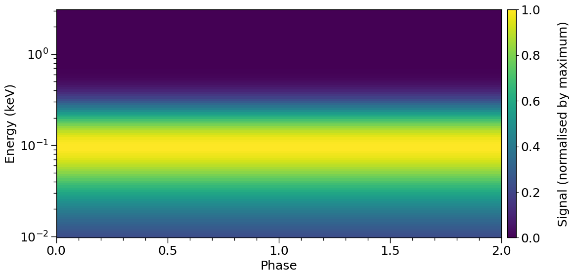
Let’s compute the incident specific flux signal, up to some constant coefficient.
[10]:
energies = np.logspace(-2.0, np.log10(3.0), 100, base=10.0)
[11]:
photosphere.integrate(energies=energies, threads=4)
The signal is time-invariant and therefore we need to copy the spectrum to a sequence of matrix columns to get the desired energy-phase signal matrix:
[12]:
temp = np.tile(photosphere.signal[0][0], (1,100))
We need a helper function to plot the signal, normalised to the maximum specific flux:
[13]:
plot_2D_pulse(temp,
              x=np.linspace(0.0, 1.0, 100),
              shift=np.array([0.0]),
              y=energies,
              num_rotations=2.0,
              ylabel=r'Energy (keV)')
/tmp/ipykernel_7218/2055479655.py:46: DeprecationWarning: Conversion of an array with ndim > 0 to a scalar is deprecated, and will error in future. Ensure you extract a single element from your array before performing this operation. (Deprecated NumPy 1.25.)
  interpolated = phase_interpolator(new_phases,
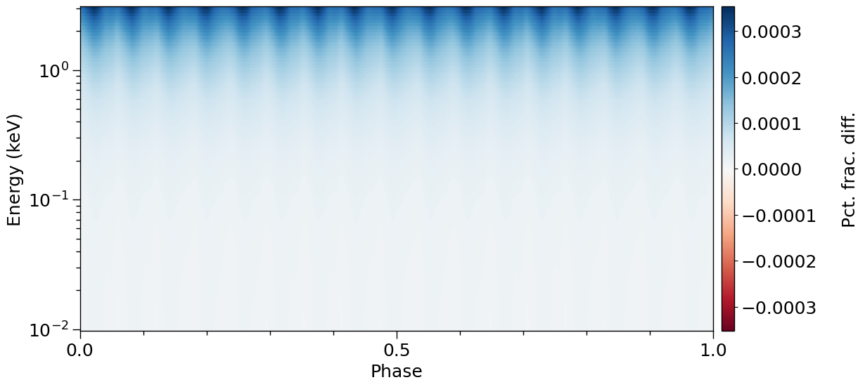
If we declare the signal as time-dependent, a different integrator is called:
[14]:
everywhere.time_invariant = False
everywhere.set_phases(512,100,None)
[15]:
photosphere.integrate(energies=energies, threads=4)
[16]:
plot_2D_pulse((photosphere.signal[0][0], temp),
              x=everywhere.phases_in_cycles,
              shift=0.0,
              y=energies,
              ylabel=r'Energy (keV)',
              cm=cm.RdBu,
              label=r"Pct. frac. diff.",
              num_rotations=1.0,
              error=True)
We can also call a third integrator. This integrator is more general purpose, and thus inexorably more expensive to call. First we need to force the spacetime to be static (otherwise univeral relations are invoked based on the stellar spin frequency as set above):
[17]:
spacetime.a = 0.0 # spacetime spin parameter (~angular momentum)
spacetime.q = 0.0 # spacetime mass quadrupole moment
Now we call the integrator. The integrator discretises a distant image plane instead of the stellar surface. The image of the star is spatially resolved on the image plane. The integrator yields four-dimensional information about the signal. We trace a set of rays from the image plane to the star; the set is roughly equal in cardinality to the number of cells that discretise the surface above. Note that when this extension module is called, some output for diagnostics is directed to the terminal in which you launched this Jupyter notebook.
If you are uninterested in generating images, you can deactivate caching of the photon specific intensity fields on the sky, which dominates memory consumption. Actually, this is the default behaviour. If you activate caching of intensities and declare that you have enough memory for X-PSI to use (see the method docstring), note that this call below could consume up to ~15 GB of RAM, and you would be forced to reduce the number of energies, phases, and/or rays to proceed if this is problematic. Alternatively, if you want to examine convergence of integrators, and want images, you will need to tune up resolution settings, and then you do the calculations on a so-called fat node of a high-performance system that offers increased OpenMP parallelism and crucially, a higher memory bank.
[18]:
class CustomPhotospherePlotter(xpsi.PhotospherePlotter):
    """ Implement method for imaging."""

    @property
    def global_variables(self):
        """ This method is needed if we also want to invoke the image-plane signal simulator. """

        return np.array([0.0, #self['p__super_colatitude'],
                          0.0, #self['p__phase_shift'] * 2.0 * math.pi,
                          np.pi, #self['p__super_radius'],
                          0.0, #self['p__cede_colatitude'],
                          0.0, #self['p__phase_shift'] * 2.0 * math.pi - self['p__cede_azimuth'],
                          0.0, #self['p__cede_radius'],
                          0.0, #self['s__super_colatitude'],
                          0.0, #(self['s__phase_shift'] + 0.5) * 2.0 * math.pi,
                          0.0, #self['s__super_radius'],
                          0.0, #self['s__cede_colatitude'],
                          0.0, #(self['s__phase_shift'] + 0.5) * 2.0 * math.pi - self['s__cede_azimuth'],
                          0.0, #self['s__cede_radius'],
                          self.photosphere['temperature'], #self['p__super_temperature'],
                          0.0, #self['p__cede_temperature'],
                          0.0, #self['s__super_temperature'],
                          0.0]) #self['s__cede_temperature']])
[19]:
plotter = CustomPhotospherePlotter(photosphere)
plotter.image(reimage = True,
                  energies = energies,
                  phases = everywhere.phases_in_cycles * _2pi,
                  sqrt_num_rays = 512,
                  threads = 4,          # OpenMP
                  max_steps = 100000,   # max number of steps per ray
                  epsrel_ray = 1.0e-12) # ray relative tolerance
[Coordinate frequency of the mode of radiative asymmetry in the
photosphere that is assumed to generate the pulsed signal [Hz] = 6.000e+02, log10(effective temperature [K] everywhere) = 6.000e+00]
Imaging the star...
Warning: a ray map has not been cached... tracing new ray set...
Commencing ray tracing and imaging...
Imaging the star and computing light-curves...
Calculating image plane boundary...
Image plane semi-major: 1.00
Image plane semi-minor: 1.00
Thread 0 is tracing annulus #0 of rays.
Warning: cosine aberrated surface zenith angle = 1.00000033e+00...
Warning: forcing the aberrated ray to be normal.
Thread 0 is tracing annulus #100 of rays.
Thread 0 is tracing annulus #200 of rays.
Thread 0 is tracing annulus #300 of rays.
Thread 0 is tracing annulus #400 of rays.
Thread 0 is tracing annulus #500 of rays.

Global ray map computed.
Coordinates transformed from Boyer-Lindquist to spherical.
Commencing imaging...Ray tracing complete.
Ray set cached.
Phase-resolved specific flux integration complete.
Star imaged.
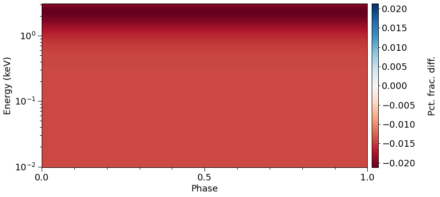
We now compare the signal to those computed above. The phase-energy resolved specific flux signal (integrated over sky solid angle) can be accessed through the images property of the photosphere object. The elements of this property also contain image plane coordinates, stellar surface coordinates, and quantities such as the specific photon intensity as a function of phase, energy, and sky direction (image plane coordinates). Note that the units of the specific flux signal are
photons/cm\(^{2}\)/s/keV because it has already been scaled by the square of the distance. The signals generated by the integrators above have not been scaled by the square of the distance (an implementation specific detail that is susceptible to change in the future).
[20]:
plot_2D_pulse((plotter.images[0]*spacetime.d_sq, temp),
              x=everywhere.phases_in_cycles,
              shift=0.0,
              y=energies,
              ylabel=r'Energy (keV)',
              cm=cm.RdBu,
              label=r"Pct. frac. diff.",
              num_rotations=1.0,
              error=True)
[21]:
fig = plt.figure(figsize=(10,10))

ax = fig.add_subplot(211)

ax.plot(energies,
         temp[:,0]/np.max(temp[:,0]),
         'k-')

ax.plot(energies,
         photosphere.signal[0][0][:,0]/np.max(temp[:,0]),
         'k--')

ax.plot(energies,
         plotter.images[0][:,0]*spacetime.d_sq/np.max(temp[:,0]),
         'k-.')

ax.set_xscale('log')
ax.set_ylabel(r'Normalised photons/cm$^{2}$/s/keV')
ax.set_yscale('log')
ax.xaxis.set_ticklabels([])
veneer((None, None), (None, None), ax)

ax = fig.add_subplot(212)

ax.plot(energies,
         100.0*np.abs(photosphere.signal[0][0][:,0]/temp[:,0] - 1.0),
         'k--')

ax.plot(energies,
         100.0*np.abs(plotter.images[0][:,0]*spacetime.d_sq/temp[:,0] - 1.0),
         'k-.')

ax.set_xscale('log')
ax.set_xlabel('Energy [keV]')

ax.set_yscale('log')
ax.set_ylabel('Abs. % frac. diff.')

veneer((None, None), (None, None), ax)

plt.subplots_adjust(hspace=0.1)
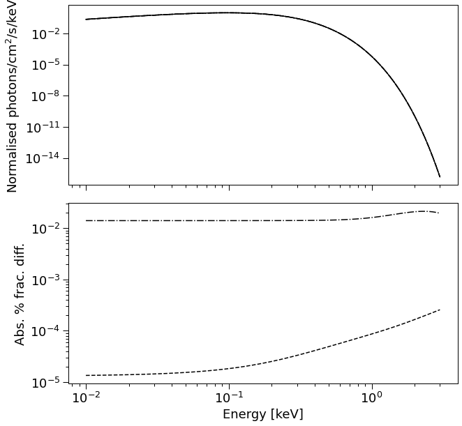
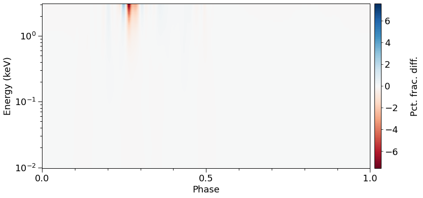
The differences can be reduced, within the scope of a given algorithm, by defining higher resolution integration settings. The integration algorithms are so distinct that this consistency validates the tools internally; verification against external packages would nevertheless permit stronger guarantees of robustness. The simple package rayXpanda offered a weak validation of the Schwarzschild ray integration routines called by the surface-discretisation signal integrators.
Let’s visualise the distribution of rays, and thus the discretisation pattern on the image plane.
[22]:
# shape into (elliptical) rings and (quasi-linear) spokes
x = plotter.images[1][1:].reshape(512,512)
y = plotter.images[2][1:].reshape(512,512)

x_origin = plotter.images[1][0]
y_origin = plotter.images[2][0]
[23]:
fig = plt.figure(figsize=(10,10))

plt.scatter(x_origin, y_origin, color='k', marker='+')
 # stride through rings and spokes
plt.scatter(x[::8,::8], y[::8,::8], s=0.1, color='k', marker='.')
plt.plot(x[-1,:], y[-1,:], color='k', linewidth=0.5)

ax = plt.gca()
ax.set_xlim([-1.025,1.025])
ax.set_ylim([-1.025,1.025])
veneer((0.05,0.25), (0.05,0.25), ax)
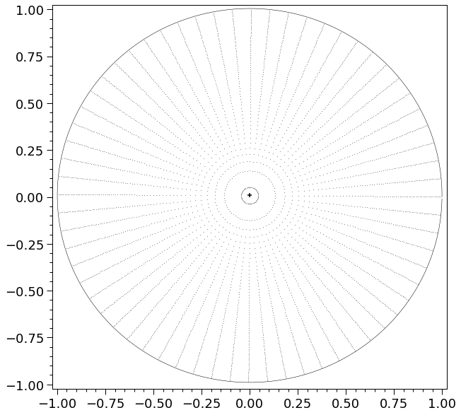
Notice that the rays are squeezed towards the stellar limb. The origin of the ray pattern, and the outer boundary are such that the image of the star is efficiently and accurately bounded with minimal ray wastage.
Let’s plot a photon specific intensity sky map, with the surface coordinates and ray pattern overplotted. We thus need to cache intensities when we integrate, so let’s choose a few energies and fewer rays to reduce memory requirements by a factor of \(\sim\!25\):
[24]:
plotter.image(reimage = True,
                  cache_intensities = 1.0, # cache size limit in GBs
                  energies = np.array([0.01,0.1,0.5,1.0,2.0,5.0]),
                  phases = everywhere.phases_in_cycles * _2pi,
                  sqrt_num_rays = 400,
                  threads = 4,
                  max_steps = 100000,
                  epsrel_ray = 1.0e-12)
Imaging the star...
Cached ray set to be reused... commencing imaging...
Imaging the star and computing light-curves...
Commencing imaging...Intensity caching complete.
Star imaged.
[25]:
plotter.plot_sky_map()
The contour artefact is seemingly unavoidable due to the wrapping of the azimuthal coordinate; one can put the boundary (beyond which \(\phi\mapsto\phi-2\pi\)) at different azimuths, but in matplotlib the thick dark contour mass remains (here visible at the northern and southern rotation poles).
Let’s generate the photon specific intensity sky maps at a set of energies, and optionally an animated compilation of those images.
[26]:
sky_map_kwargs = {'panel_indices': (0,1,2,3,4,5), # select energy indexes
                  'num_levels': 500,
                  'colormap': cm.Purples_r,
                  'phase_average': True,
                  'annotate_energies': True,
                  'energy_annotation_format': '[%.2f keV]',
                  'annotate_location': (0.025,0.025)} # do not phase average if you want to animate a sequence
NB: a colormap like cm.Purples_r this will make the lowest finite intensity distinct from the black zero-intensity background from the surface and behind the star.
[27]:
plotter.image(reimage = False,
              energies = np.array([0.01,0.1,0.5,1.0,2.0,5.0]),
              phases = everywhere.phases_in_cycles * _2pi,
              generate_sky_maps = True,
              sky_map_kwargs = sky_map_kwargs,
              animate_sky_maps = False,
              animate_kwargs = {})
Imaging the star...
Plotting intensity sky maps...
Averaging (specific) intensity over rotational phase...
Averaged (specific) intensity over rotational phase.
Normalising each sky map panel separately...
Normalised sky map panels separately.
Rendering phase-averaged images...
Intensity sky maps plotted.
Star imaged.
Let’s display a set of sky phase-averaged maps (which are identical to the phase-resolved maps for this axisymmetric surface radiation field specification):
[28]:
Image("./images/skymap_0.png")
[28]:
[29]:
!mkdir images/uniform
!mv images/skymap_0.png images/uniform/skymap_default.png
mkdir: cannot create directory ‘images/uniform’: File exists
With that out of the way, let’s explore a surface radiation field whose spatial structure exhibits higher-complexity.
Custom (phase-dependent)
Let us, inspired by Lockhart et al. (2019), set up a surface radiation field constituted by: (i) a hot spot whose temperature decreases away from a point \(P\) as a function of angular separation; and (ii) a hot ring whose angular centre is the antipode \(Q\) of \(P\) and whose temperature decreases away (as a function of angular separation from \(Q\)) from a locus of points with constant angular separation to point \(Q\). The temperature is everywhere that of the local comoving photosphere, which radiates isotropically as a blackbody.
You now need to reinstall the package after replacing the contents of ``xpsi/surface_radiation_field/local_variables.pyx`` with the exact contents of ``xpsi/surface_radiation_field/archive/local_variables/tutorial_spot_and_ring.pyx``. The local_variables.pyx extension module must transform some set of global variables into local variables at the spacetime event defined by the intersection of a ray with the stellar surface. A vector of local variables is then passed to the
xpsi/surface_radiation_field/hot.pyx module for evaluation of the specific intensity of radiation, w.r.t a local comoving surface frame, that after Lorentz transformation is transported along the ray to the image plane.
Once you can reinstalled the package, you need to restart the IPython kernel and then execute code cells [1], [2], and [3] above.
First we will subclass Everywhere to provide a custom implementation of the surface radiation field for a surface-discretisation integrator.
[4]:
class CustomEverywhere(xpsi.Everywhere):
    """ Custom radiation field globally spanning the surface. """

    @classmethod
    def create_parameters(cls, bounds, values={}, *args, **kwargs):
        """ Create custom parameter objects. """

        T = Parameter('spot_temperature',
                      strict_bounds = (3.0, 7.0), # very cold --> very hot
                      bounds = bounds.get('spot_temperature', None),
                      doc = 'log10(spot temperature [K])',
                      symbol = r'$\log_{10}(T\;[\rm{K}])$',
                      value = values.get('spot_temperature', None))

        colatitude = Parameter('colatitude',
                               strict_bounds = (0.0, math.pi),
                               bounds = bounds.get('colatitude', None),
                               doc = 'spot centre colatitude [radians]',
                               symbol = r'$\Theta$',
                               value = values.get('colatitude', None))

        spot_scale = Parameter('spot_scale',
                               strict_bounds = (0.0, math.pi/2.0),
                               bounds = bounds.get('spot_scale', None),
                               doc = 'scale of temperature variation [radians]',
                               symbol = r'$\sigma$',
                               value = values.get('spot_scale', None))

        rotation = Parameter('rotation',
                             strict_bounds = (0.0, 2.0*math.pi),
                             bounds = bounds.get('rotation', None),
                             doc = 'stellar rotation [radians]',
                             symbol = r'$\phi$',
                             value = values.get('rotation', None))

        return cls(*args,
                   custom=[T,
                           colatitude,
                           spot_scale,
                           rotation],
                           **kwargs)

    @staticmethod
    def angular_separation(theta, phi, colatitude):
        """ Colatitude in rotated basis (anti-clockwise about y-axis). """
        return xpsi.HotRegion.psi(theta, phi, colatitude)

    def _compute_cellParamVecs(self):
        """ Custom temperature field variation to imitate hot spot + ring. """
        # all radiate, but can be changed with overwrite
        self._cellRadiates = np.ones(self._theta.shape, dtype=np.int32)

        separation = self.angular_separation(self._theta, self._phi, self['colatitude'])

        self._cellParamVecs = np.ones((self._theta.shape[0],
                                        self._theta.shape[1],
                                        2), dtype=np.double)

        self._cellParamVecs[...,0] = self['spot_temperature'] * np.exp(-(separation-self['spot_scale'])**2.0/(2.0*0.25*self['spot_scale']))
        self._cellParamVecs[...,0] += self['spot_temperature'] * np.exp(-(separation-math.pi)**2.0/(2.0*self['spot_scale']))

        for i in range(self._cellParamVecs.shape[1]):
            self._cellParamVecs[:,i,-1] *= self._effGrav # unused here

        self._phi += self['rotation']
[5]:
bounds = dict(spot_temperature = (5.5, 6.5),
              colatitude = (None, None),
              spot_scale = (None, None),
              rotation = (None, None))

everywhere = CustomEverywhere.create_parameters(bounds=bounds,
                values={},            # no fixed/derived variables
                time_invariant=False, # choose appropriate integrator
                sqrt_num_cells=512,
                num_rays=1000,
                num_leaves=512,
                num_phases=100)
Creating parameter:
    > Named "spot_temperature" with bounds [5.500e+00, 6.500e+00].
    > log10(spot temperature [K]).
Creating parameter:
    > Named "colatitude" with bounds [0.000e+00, 3.142e+00].
    > spot centre colatitude [radians].
Creating parameter:
    > Named "spot_scale" with bounds [0.000e+00, 1.571e+00].
    > scale of temperature variation [radians].
Creating parameter:
    > Named "rotation" with bounds [0.000e+00, 6.283e+00].
    > stellar rotation [radians].
Creating parameter:
    > Named "phase_shift" with fixed value 0.000e+00.
We want to image the photosphere and the default behaviour of Photosphere is insufficient. We therefore subclass Photosphere to provide a custom implementation of a higher-complexity radiation field. The customisation is actually very simple: we must make a property return a vector of global variable values that are relayed to a compiled extension module
xpsi.surface_radiation_field.local_variables by the image-plane discretisation integrator. Thus, the bulk of the customisation must be written in xpsi/surface_radiation_field/local_variables.pyx for compilation; this has already been handled for this tutorial (see instructions above).
[6]:
photosphere = xpsi.Photosphere(hot = None,
                                elsewhere = None,
                                everywhere = everywhere,
                                values=dict(mode_frequency = spacetime['frequency']))
Creating parameter:
    > Named "mode_frequency" with fixed value 6.000e+02.
    > Coordinate frequency of the mode of radiative asymmetry in the
photosphere that is assumed to generate the pulsed signal [Hz].
[7]:
star = xpsi.Star(spacetime = spacetime, photospheres = photosphere)
[8]:
def set_defaults():
    global star # for clarity

    star['distance'] = 0.3

    star['mass'] = 2.0

    star['radius'] = 12.0

    star['cos_inclination'] = math.cos(1.0)

    star['spot_temperature'] = 6.2

    star['colatitude'] = 3.0 * math.pi/4.0

    star['spot_scale'] = 0.5

    star['rotation'] = math.pi/2.0

set_defaults()
[9]:
star.update()
[10]:
energies = np.logspace(-2.0, np.log10(3.0), 100, base=10.0)
[11]:
photosphere.integrate(energies=energies, threads=4)
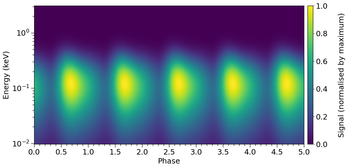
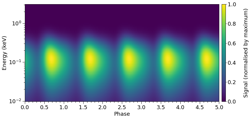
[12]:
plot_2D_pulse(photosphere.signal[0][0],
              x=everywhere.phases_in_cycles,
              shift=0.0,
              y=energies,
              ylabel=r'Energy (keV)')
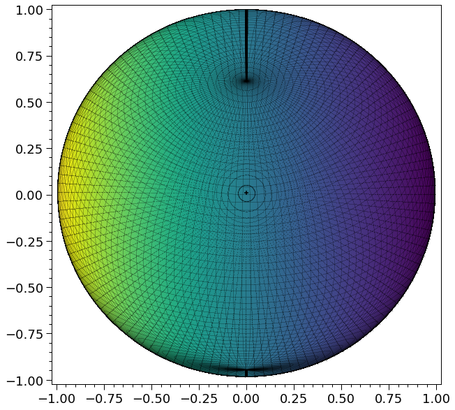
Let’s render the surface temperature field represented by our regular mesh in colatitude and azimuth:
[13]:
fig = plt.figure(figsize = (10,10))

ax = fig.add_subplot(111)
veneer((20, 100), (20, 100), ax)

z = everywhere._cellParamVecs[...,0]
patches = plt.imshow(z, rasterized = True)
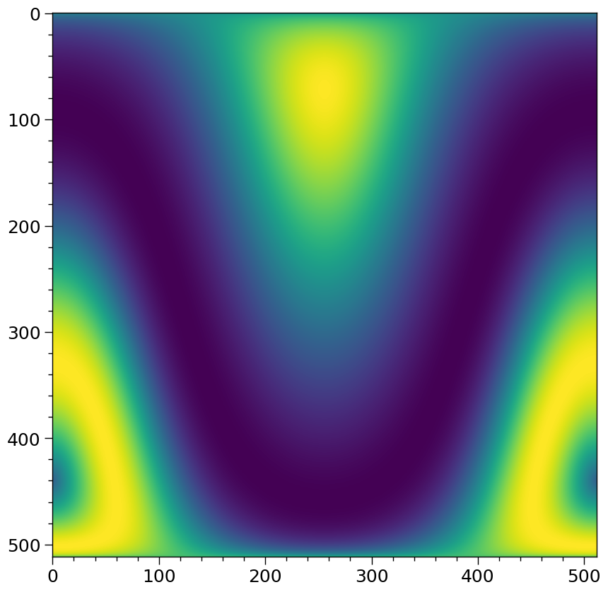
Colatitude increases downwards, whilst azimuth increases rightwards. The mesh is constructed such that the \(\phi\mapsto\phi-2\pi\) boundary is the meridian on which the angular centre of the ring lies. We can make a crude plot of the surface temperature field in a more natural way:
[14]:
#This code block (if uncommented) currently results in
#"ValueError: cannot reshape array of size 0 into shape (0,newaxis)"
#if using matplotlib version 3.9.2.
#The reason for this is being investigated.

# plt.figure(figsize=(10,10))
# plt.subplot(111, projection="lambert")

# plt.grid(True)

# Lat = -everywhere._theta + math.pi/2.0

# z = everywhere._cellParamVecs[...,0]

# plt.contour(everywhere._phi, Lat, z,
#            levels=np.linspace(np.min(z), np.max(z), 50))

# _ = plt.gca().set_xticklabels([])
Note that although the star looks lensed, it is merely a projection (mimicking Schwarzschild light bending for an equatorial observer) that allows us to render all \(4\pi\) steradians of the surface. The real lensing is yet to come! First we need to force our exterior spacetime to be that of Schwarzschild:
[15]:
spacetime.a = 0.0 # spacetime spin parameter (~angular momentum)
spacetime.q = 0.0 # spacetime mass quadrupole moment
Now call the imaging routine in the same manner as above:
[16]:
class CustomPhotospherePlotter(xpsi.PhotospherePlotter):
    """ Implement custom global variables property. """

    @property
    def global_variables(self):
        return np.array([self.photosphere['spot_temperature'],
                         self.photosphere['colatitude'],
                         self.photosphere['spot_scale'],
                         self.photosphere['rotation']])
[17]:
plotter = CustomPhotospherePlotter(photosphere)
plotter.image(reimage = True,
                  energies = energies,
                  phases = everywhere.phases_in_cycles * _2pi,
                  sqrt_num_rays = 1000, # because why not?
                  threads = 4,
                  max_steps = 100000,
                  epsrel_ray = 1.0e-12)
[Coordinate frequency of the mode of radiative asymmetry in the
photosphere that is assumed to generate the pulsed signal [Hz] = 6.000e+02, log10(spot temperature [K]) = 6.200e+00, spot centre colatitude [radians] = 2.356e+00, scale of temperature variation [radians] = 5.000e-01, stellar rotation [radians] = 1.571e+00]
Imaging the star...
Warning: a ray map has not been cached... tracing new ray set...
Commencing ray tracing and imaging...
Imaging the star and computing light-curves...
Calculating image plane boundary...
Image plane semi-major: 1.00
Image plane semi-minor: 1.00
Thread 0 is tracing annulus #0 of rays.
Warning: cosine aberrated surface zenith angle = 1.00000002e+00...
Warning: forcing the aberrated ray to be normal.
Thread 0 is tracing annulus #100 of rays.
Thread 0 is tracing annulus #200 of rays.
Thread 0 is tracing annulus #300 of rays.
Thread 0 is tracing annulus #400 of rays.
Thread 0 is tracing annulus #500 of rays.
Warning: cosine aberrated surface zenith angle = -1.39209632e-03...
Warning: forcing the aberrated ray to be tangential.
Warning: cosine aberrated surface zenith angle = -1.74526434e-03...
Warning: forcing the aberrated ray to be tangential.
Thread 0 is tracing annulus #600 of rays.
Thread 0 is tracing annulus #700 of rays.
Thread 0 is tracing annulus #800 of rays.
Thread 0 is tracing annulus #900 of rays.

Global ray map computed.
Coordinates transformed from Boyer-Lindquist to spherical.
Commencing imaging...Ray tracing complete.
Ray set cached.
Phase-resolved specific flux integration complete.
Star imaged.
Let’s examine the phase-energy resolved photon specific flux signal and compare it to the signal computed by via surface discretisation:
[18]:
plot_2D_pulse(np.ascontiguousarray(plotter.images[0]),
              x=everywhere.phases_in_cycles,
              shift=0.0,
              y=energies,
              ylabel=r'Energy (keV)')
[19]:
plot_2D_pulse((plotter.images[0]*spacetime.d_sq, photosphere.signal[0][0]),
              x=everywhere.phases_in_cycles,
              shift=0.0,
              y=energies,
              ylabel=r'Energy (keV)',
              cm=cm.RdBu,
              label=r"Pct. frac. diff.",
              num_rotations=1.0,
              error=True)
Now the really fun part: photon specific intensity sky maps. Now that we are not pursuing a high-resolution signal to compare to an integrator that discretises the stellar surface, we reduce the number of energies and rays to avoid memory issues when caching the sky photon specific intensity field in four dimensions. Nevertheless, if you run these cells as is, you might want to grab a beverage of choice while you wait up to ~30 minutes. In previous X-PSI versions, the animator required massive memory due to matplotlib imshow() usage issues, but this was fixed in X-PSI v0.6; nevertheless, you could start with a smaller number of phases, just to check that it works without eating more memory than you want to spare.
[20]:
sky_map_kwargs = {'panel_indices': (0,1,2,3,4,5),
                  'num_levels': 100, # in intensity field rendering
                  'colormap': cm.Greys_r,
                  'phase_average': False,
                  'annotate_energies': True,  # background from the surface and behind the star
                  'energy_annotation_format': '[%.2f keV]',
                  'annotate_location': (0.025,0.025)}

# you can install ffmpeg with conda in order to animate
animate_kwargs = {'cycles': 4, 'fps': 32}
[21]:
!rm images/*.png
rm: cannot remove 'images/*.png': No such file or directory
[22]:
plotter.image(reimage = True,
                  reuse_ray_map = False,
                  cache_intensities = 1.0, # cache size limit in GBs
                  energies = np.array([0.01,0.1,0.5,1.0,2.0,5.0]),
                  phases = everywhere.phases_in_cycles * _2pi,
                  sqrt_num_rays = 400,
                  threads = 4,
                  max_steps = 100000,
                  epsrel_ray = 1.0e-12,
                  generate_sky_maps = True, # activate if you want to plot frames
                  sky_map_kwargs = sky_map_kwargs,
                  animate_sky_maps = True, # activate if you want to animate
                  free_memory = False, # activate if memory is a concern, then ray-map/intensity caches deleted
                  animate_kwargs = animate_kwargs)
Imaging the star...
Commencing ray tracing and imaging...
Imaging the star and computing light-curves...
Calculating image plane boundary...
Image plane semi-major: 1.00
Image plane semi-minor: 1.00
Thread 0 is tracing annulus #0 of rays.
Thread 0 is tracing annulus #100 of rays.
Thread 0 is tracing annulus #200 of rays.
Thread 0 is tracing annulus #300 of rays.

Global ray map computed.
Coordinates transformed from Boyer-Lindquist to spherical.
Commencing imaging...Ray tracing complete.
Ray set cached.
Intensity caching complete.
Plotting intensity sky maps...
Normalising each sky map panel separately...
Normalised sky map panels separately.
Rendering image numbers [1, 10]...
Rendering image numbers (10, 20]...
Rendering image numbers (20, 30]...
Rendering image numbers (30, 40]...
Rendering image numbers (40, 50]...
Rendering image numbers (50, 60]...
Rendering image numbers (60, 70]...
Rendering image numbers (70, 80]...
Rendering image numbers (80, 90]...
Rendering image numbers (90, 100]...
Intensity sky maps plotted.
Animating intensity sky maps...
Writing to disk: ./images/skymap_animated.mp4...
Intensity sky maps animated.
Star imaged.
If you are executing this notebook, you can view the video file:
[23]:
%%HTML
<div align="middle">
<video width="100%" controls loop>
    <source src="images/skymap_animated.mp4" type="video/mp4">
</video></div>
[24]:
!mkdir images/frames_ring_and_spot
!mv images/*.png images/frames_ring_and_spot/.
mkdir: cannot create directory ‘images/frames_ring_and_spot’: File exists
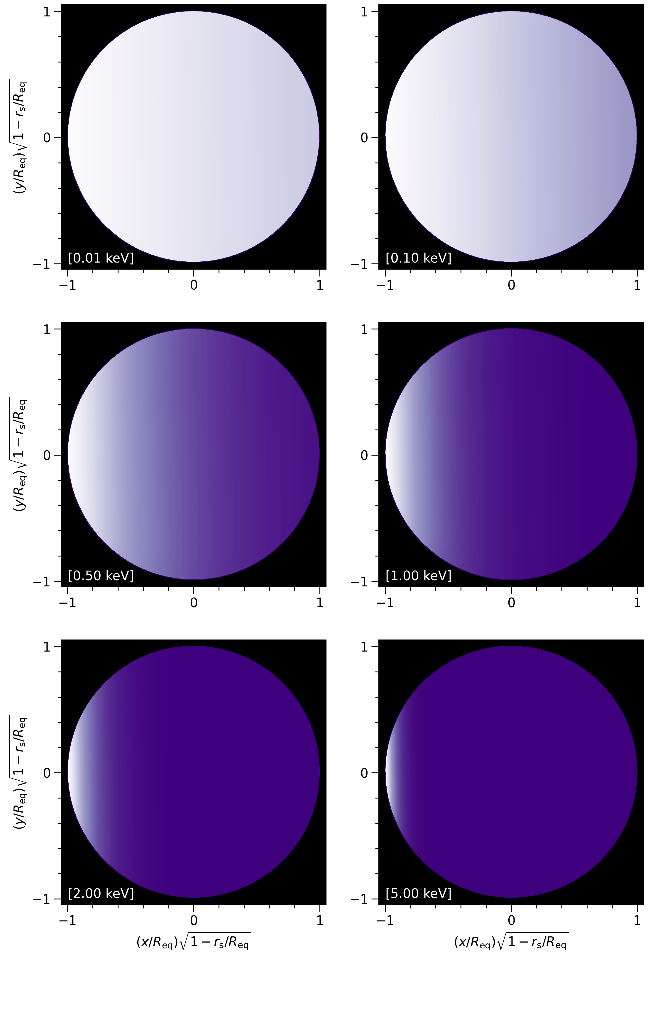
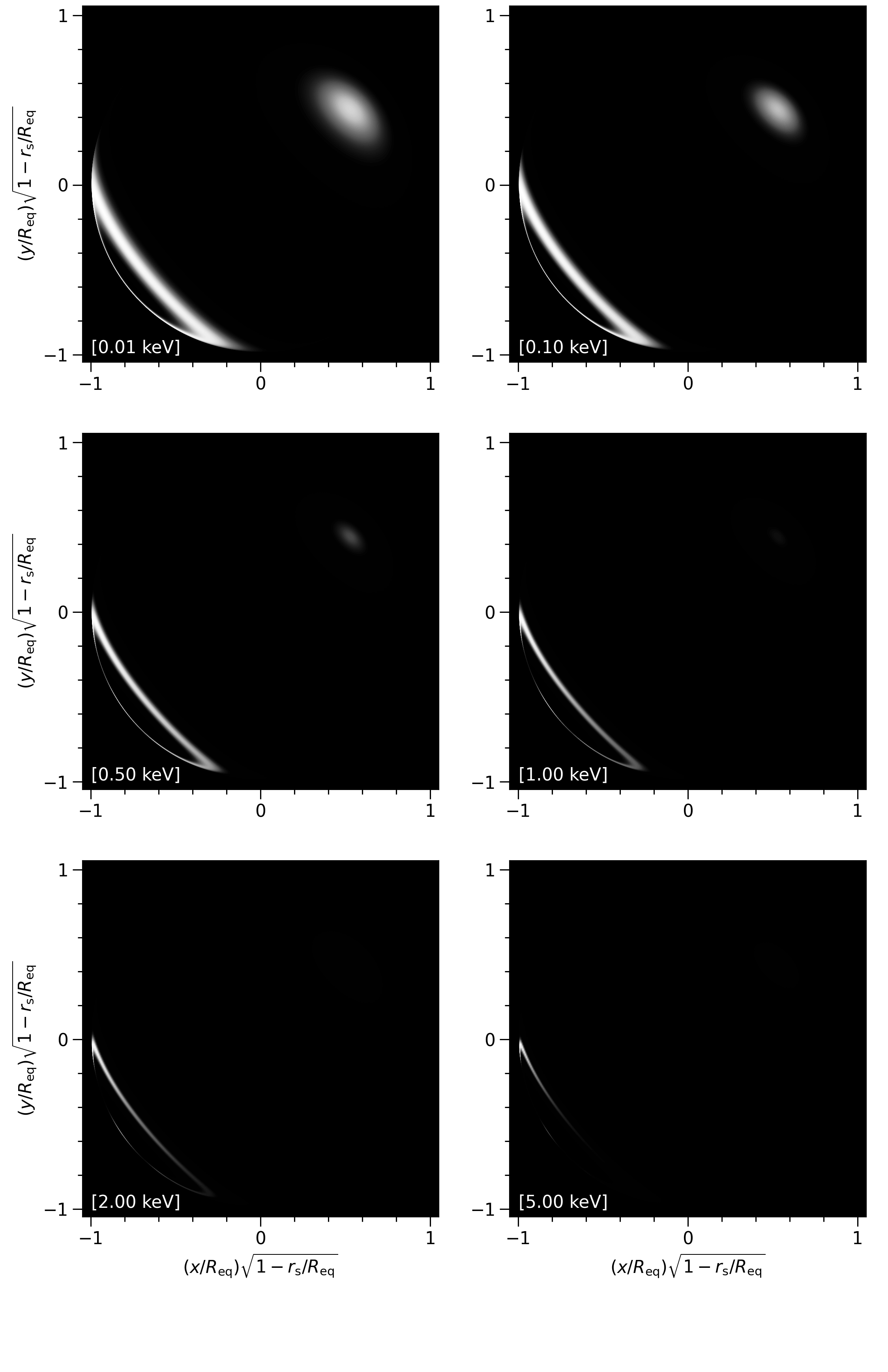
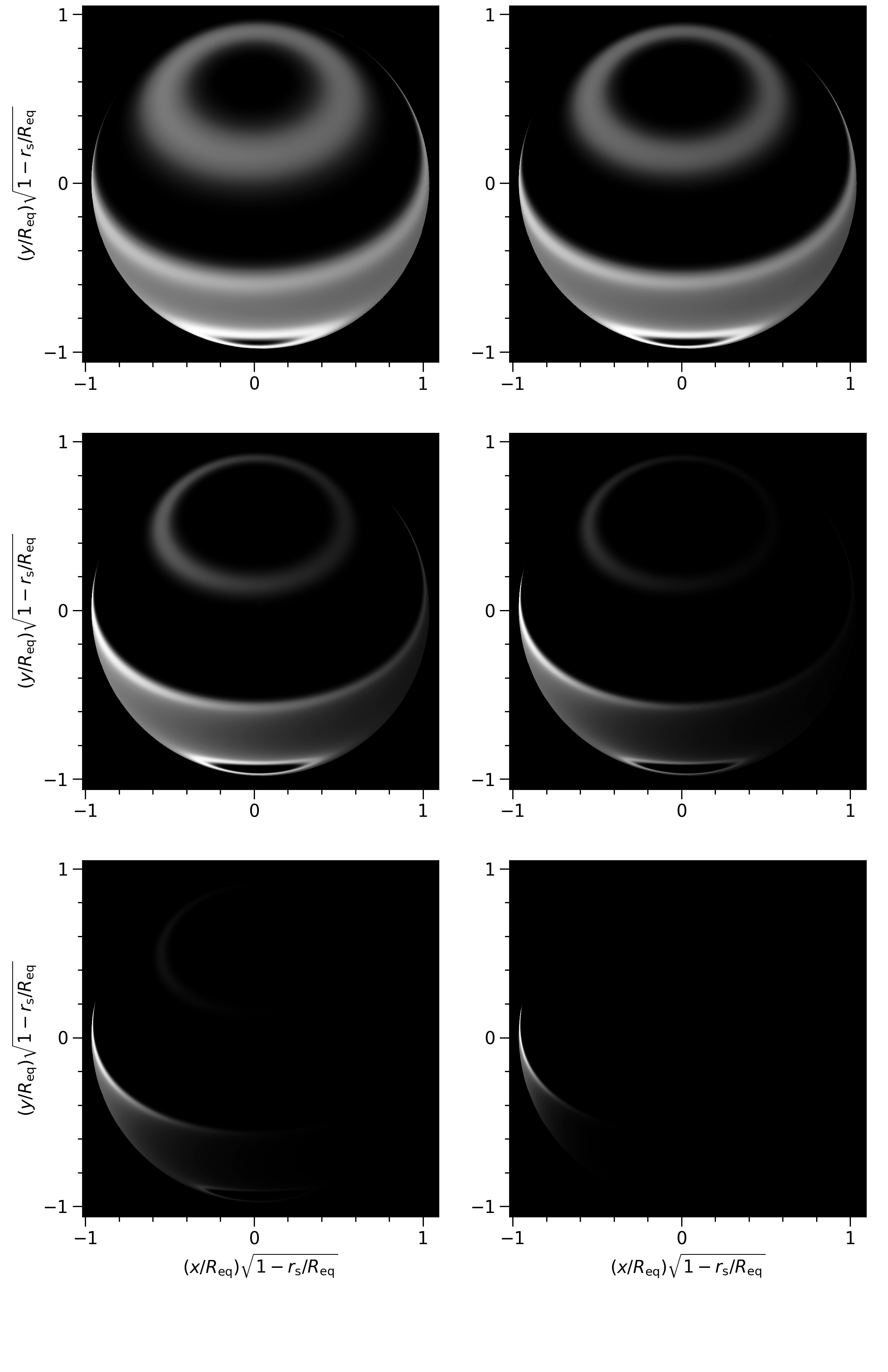
Here is a frame for the purpose of the documentation notebook. Each panel displays the photon specific intensity field, on the sky, at a given energy; energy increases from top-left to bottom-right. The intensity field in each panel is normalised over sky direction and phase, for each energy in the sequence.
[25]:
Image("./images/frames_ring_and_spot/skymap_50.png")
[25]:
Finally, let’s phase-average the intensity sky maps:
[26]:
sky_map_kwargs['phase_average'] = True
# only one set of panels so why not choose higher res.?
sky_map_kwargs['num_levels'] = 500

plotter.image(reimage = False, # because we decided not to free_memory earlier
                  energies = np.array([0.01,0.1,0.5,1.0,2.0,5.0]),
                  phases = everywhere.phases_in_cycles * _2pi,
                  generate_sky_maps = True,
                  sky_map_kwargs = sky_map_kwargs)
Imaging the star...
Plotting intensity sky maps...
Averaging (specific) intensity over rotational phase...
Averaged (specific) intensity over rotational phase.
Normalising each sky map panel separately...
Normalised sky map panels separately.
Rendering phase-averaged images...
Intensity sky maps plotted.
Star imaged.
[27]:
!mv images/skymap_0.png images/frames_ring_and_spot/skymap_phase_averaged_spot_and_ring.png
[28]:
Image("images/frames_ring_and_spot/skymap_phase_averaged_spot_and_ring.png")
[28]:

To understand the phase-averaged intensity field associated with the ring, consider a fix sky direction through which the upper and lower extremities (in colatitude) of the ring pass as the star rotates. The bright surface regions pass over such sky directions for a greater fraction of the one revolution than for sky directions closer in surface colatitude to the centre of the ring.
Rotating spacetime
The integrator that discretises an image plane, being more general purpose (but not as general purpose as a number of other open-source codes), can also handle a rotating spacetime via a CPU-based implementation of the quasi-Kerr formalism Psaltis & Johannsen (2012) and Bauböck et al. (2012), in which the exterior spacetime solution has a finite angular momentum and mass quadrupole moment. If we delete the custom values of these spacetime variables, universal relations from AlGendy & Morsink (2014) will be invoked.
[29]:
del spacetime.a
del spacetime.q
[30]:
spacetime.a # dimensions of length
[30]:
765.8499186550695
[31]:
spacetime.q # dimensionless
[31]:
0.1146198823594334
[32]:
sky_map_kwargs = {'panel_indices': (0,1,2,3,4,5),
                  'num_levels': 500, # in intensity field rendering
                  'colormap': cm.Greys_r,
                  'phase_average': True}

plotter.image(reimage = True,
                  reuse_ray_map = False, # have to do manually because free parameters have not changed
                  cache_intensities = 1.0, # cache size limit in GBs
                  energies = np.array([0.01,0.1,0.5,1.0,2.0,5.0]),
                  phases = everywhere.phases_in_cycles * _2pi,
                  sqrt_num_rays = 400,
                  threads = 4,
                  max_steps = 100000,
                  epsrel_ray = 1.0e-12,
                  generate_sky_maps = True,
                  sky_map_kwargs = sky_map_kwargs)
Imaging the star...
Commencing ray tracing and imaging...
Imaging the star and computing light-curves...
Calculating image plane boundary...
Image plane semi-major: 1.00
Image plane semi-minor: 0.99
Thread 0 is tracing annulus #0 of rays.
Warning: cosine aberrated surface zenith angle = 1.00000422e+00...
Warning: forcing the aberrated ray to be normal.
Warning: cosine aberrated surface zenith angle = 1.00001894e+00...
Warning: forcing the aberrated ray to be normal.
Warning: cosine aberrated surface zenith angle = 1.00002438e+00...
Warning: forcing the aberrated ray to be normal.
Warning: cosine aberrated surface zenith angle = 1.00001930e+00...
Warning: forcing the aberrated ray to be normal.
Warning: cosine aberrated surface zenith angle = 1.00000471e+00...
Warning: forcing the aberrated ray to be normal.
Warning: cosine aberrated surface zenith angle = 1.00002770e+00...
Warning: forcing the aberrated ray to be normal.
Warning: cosine aberrated surface zenith angle = 1.00005165e+00...
Warning: forcing the aberrated ray to be normal.
Warning: cosine aberrated surface zenith angle = 1.00006534e+00...
Warning: forcing the aberrated ray to be normal.
Warning: cosine aberrated surface zenith angle = 1.00006865e+00...
Warning: forcing the aberrated ray to be normal.
Warning: cosine aberrated surface zenith angle = 1.00006228e+00...
Warning: forcing the aberrated ray to be normal.
Warning: cosine aberrated surface zenith angle = 1.00004510e+00...
Warning: forcing the aberrated ray to be normal.
Warning: cosine aberrated surface zenith angle = 1.00001761e+00...
Warning: forcing the aberrated ray to be normal.
Warning: cosine aberrated surface zenith angle = 1.00002845e+00...
Warning: forcing the aberrated ray to be normal.
Warning: cosine aberrated surface zenith angle = 1.00005209e+00...
Warning: forcing the aberrated ray to be normal.
Warning: cosine aberrated surface zenith angle = 1.00006423e+00...
Warning: forcing the aberrated ray to be normal.
Warning: cosine aberrated surface zenith angle = 1.00006595e+00...
Warning: forcing the aberrated ray to be normal.
Warning: cosine aberrated surface zenith angle = 1.00005727e+00...
Warning: forcing the aberrated ray to be normal.
Warning: cosine aberrated surface zenith angle = 1.00003771e+00...
Warning: forcing the aberrated ray to be normal.
Warning: cosine aberrated surface zenith angle = 1.00000751e+00...
Warning: forcing the aberrated ray to be normal.
Warning: cosine aberrated surface zenith angle = 1.00000909e+00...
Warning: forcing the aberrated ray to be normal.
Warning: cosine aberrated surface zenith angle = 1.00002016e+00...
Warning: forcing the aberrated ray to be normal.
Warning: cosine aberrated surface zenith angle = 1.00002009e+00...
Warning: forcing the aberrated ray to be normal.
Warning: cosine aberrated surface zenith angle = 1.00000907e+00...
Warning: forcing the aberrated ray to be normal.
Thread 0 is tracing annulus #100 of rays.
Thread 0 is tracing annulus #200 of rays.
Thread 0 is tracing annulus #300 of rays.
Warning: cosine aberrated surface zenith angle = -5.02758155e-04...
Warning: forcing the aberrated ray to be tangential.

Global ray map computed.
Coordinates transformed from Boyer-Lindquist to spherical.
Commencing imaging...Ray tracing complete.
Ray set cached.
Intensity caching complete.
Plotting intensity sky maps...
Averaging (specific) intensity over rotational phase...
Averaged (specific) intensity over rotational phase.
Normalising each sky map panel separately...
Normalised sky map panels separately.
Rendering phase-averaged images...
Intensity sky maps plotted.
Star imaged.
[33]:
!mv images/skymap_0.png images/frames_ring_and_spot/skymap_phase_averaged_spot_and_ring__rotating_spacetime.png
[34]:
Image("images/frames_ring_and_spot/skymap_phase_averaged_spot_and_ring__rotating_spacetime.png")
[34]:
You should be able to detect the extra lateral asymmetry introduced at lower energies that was not present for a static ambient spacetime.
Note that the temporal and azimuthal coordinates are no longer those used above for the Schwarzschild exterior spacetime solution, and thus the surface radiation field is inherently different when the same functions of azimuthal and temporal coordinates are used to construct it.
The integrator can also handle some forms of time evolution of the surface radiation field beyond pure bulk rotation, but such a usage pattern is more advanced and thus left for a future tutorial.