Surface radiation field tools
In this tutorial we demonstrate usage of several tools for checking the implementation of a surface radiation field extension module.
For the first part of this tutorial, you should install X-PSI with the default (blackbody) atmosphere extension module, which is compiled when installing X-PSI with default settings. Then run the full the tutorial except the one code block under the title “Isotropic blackbody” after re-installing X-PSI using the numerical atmosphere extension using the NumHot and NumElse options and re-starting the IPython kernel.
The required atmosphere data files are needed and they can be found in the Zenodo.
[8]:
%matplotlib inline

import warnings
warnings.filterwarnings(action='ignore')
import numpy as np
[9]:
import xpsi
/=============================================\
| X-PSI: X-ray Pulse Simulation and Inference |
|---------------------------------------------|
|                Version: 1.0.0               |
|---------------------------------------------|
|      https://xpsi-group.github.io/xpsi      |
\=============================================/

Imported GetDist version: 0.3.1
Imported nestcheck version: 0.2.0
[10]:
from matplotlib import pyplot as plt
plt.rc('font', size=20.0)
Calculate the specific intensity directly from local variables
[11]:
# keV (local comoving frame)
E = np.logspace(-2.0, 0.5, 1000, base=10.0)

# cos(angle to local surface normal in comoving frame)
mu = np.ones(1000) * 0.5

# log10(eff. temperature [K]) and log10(local eff. gravity [cm/s^2])
local_vars = np.array([[6.11, 13.8]]*1000)
[12]:
xpsi.surface_radiation_field?
[13]:
xpsi.surface_radiation_field.intensity?
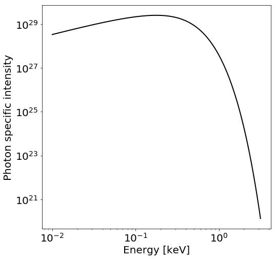
Isotropic blackbody
For the following cell, make sure you have installed X-PSI with default settings.
[7]:
plt.figure(figsize=(8,8))

BB_I = xpsi.surface_radiation_field.intensity(E, mu, local_vars, # NB: isotropic blackbody
                                              extension='elsewhere', numTHREADS=2)

plt.plot(E, BB_I, 'k-', lw=2.0)

# write it to disk so accessible upon IPython kernel restart (see below)
np.savetxt('./blackbody_spectrum_cache.txt', BB_I)

ax = plt.gca()
ax.set_yscale('log')
ax.set_xscale('log')
ax.set_ylabel('Photon specific intensity')
_ = ax.set_xlabel('Energy [keV]')
Numerical atmosphere
Let’s check out a numerical atmosphere (this code you typically find in a custom photosphere class). The numerical atmospheres loaded here were generated by the NSX atmosphere code (Ho, W.C.G & Lai, D. 2001; Ho, W.C.G & Heinke, C.O. 2009), courtesy of W.C.G. Ho for NICER modeling efforts. One of these atmospheres (fully-ionized
hydrogen; Ho & Lai 2001) was used in Riley et al. (2019); also see Bogdanov et al. (2020) and Riley et al. (2021). For this tutorial we need the data files nsx_H_v171019.out and nsx_He_v170925.out that can be found in Zenodo. The repository includes also a fully-ionized hydrogen data file with an extended surface gravity grid (nsx_H_v200804.out), which was used in Riley et al. 2021, but not
in this tutorial.
Reinstall X-PSI with the appropriate flags as such: CC=gcc python setup.py install --NumHot --NumElse (see also Installation). These flags ensure hot.pyx is replaced with archive/hot/numerical.pyx, and elsewhere.pyx is replaced by archive/elsewhere/numerical.pyx. Next, restart your IPython kernel, and run all cells above, apart from [7].
[14]:
def preload(path, size):
    NSX = np.loadtxt(path, dtype=np.double)
    logT = np.zeros(size[0])
    logg = np.zeros(size[1])
    _mu = np.zeros(size[2]) # use underscore to bypass errors with the other mu array
    logE = np.zeros(size[3])

    reorder_buf = np.zeros(size)

    index = 0
    for i in range(reorder_buf.shape[0]):
        for j in range(reorder_buf.shape[1]):
            for k in range(reorder_buf.shape[3]):
               for l in range(reorder_buf.shape[2]):
                    logT[i] = NSX[index,3]
                    logg[j] = NSX[index,4]
                    logE[k] = NSX[index,0]
                    _mu[reorder_buf.shape[2] - l - 1] = NSX[index,1]
                    reorder_buf[i,j,reorder_buf.shape[2] - l - 1,k] = 10.0**(NSX[index,2])
                    index += 1

    buf = np.zeros(np.prod(reorder_buf.shape))

    bufdex = 0
    for i in range(reorder_buf.shape[0]):
        for j in range(reorder_buf.shape[1]):
            for k in range(reorder_buf.shape[2]):
               for l in range(reorder_buf.shape[3]):
                    buf[bufdex] = reorder_buf[i,j,k,l]; bufdex += 1

    atmosphere = (logT, logg, _mu, logE, buf)

    return atmosphere
[15]:
H_fully = preload('../../examples/examples_modeling_tutorial/model_data/nsx_H_v171019.out',
                    size=(35, 11, 67, 166))
[16]:
He_fully = preload('../../examples/examples_modeling_tutorial/model_data/nsx_He_v170925.out',
                      size=(29, 11, 67, 166))
[17]:
plt.figure(figsize=(8,8))

BB_I = np.loadtxt('./blackbody_spectrum_cache.txt')
plt.plot(E, BB_I, 'k--', lw=1.0)

hot_I = xpsi.surface_radiation_field.intensity(E, mu, local_vars,
                                               atmosphere=H_fully,
                                               extension='hot',
                                               numTHREADS=2)

plt.plot(E, hot_I, 'b-', lw=2.0)

elsewhere_I = xpsi.surface_radiation_field.intensity(E, mu, local_vars,
                                                     atmosphere=H_fully,
                                                     extension='elsewhere',
                                                     numTHREADS=2)

plt.plot(E, elsewhere_I, 'r-', lw=1.0)

He_fully_I = xpsi.surface_radiation_field.intensity(E, mu, local_vars,
                                                     atmosphere=He_fully,
                                                     extension='hot',
                                                     numTHREADS=2)

plt.plot(E, He_fully_I, 'k-.', lw=1.0)

ax = plt.gca()
ax.set_yscale('log')
ax.set_ylim([9.0e25,4.0e29])
ax.set_xscale('log')
ax.set_ylabel('Photon specific intensity')
_ = ax.set_xlabel('Energy [keV]')
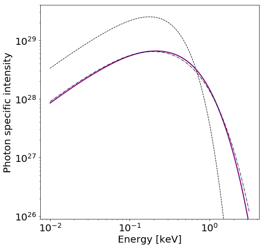
This behaviour is typical for an isotropic blackbody radiation field with temperature \(T\) in comparison to a radiation field emergent from a (non-magnetic, fully-ionized) geometrically-thin H/He atmosphere with effective temperature \(T\).
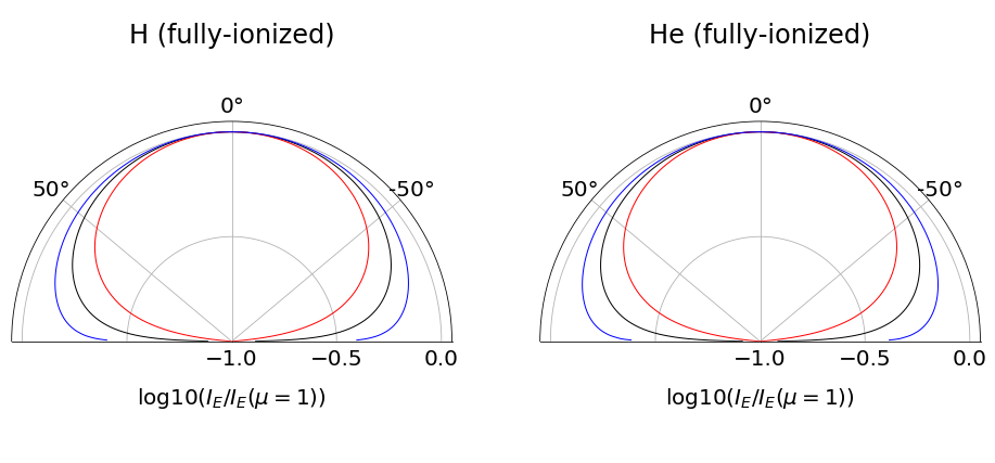
Let’s plot the angular dependence:
[18]:
# keV (local comoving frame)
E = np.ones(1000) * 0.2

# cos(angle to local surface normal in comoving frame)
mu = np.linspace(0.01,1.0,1000)

fig = plt.figure(figsize=(16,8))

# Hydrogen

ax = fig.add_subplot(121, projection='polar')

ax.set_theta_direction(1)
ax.set_thetamin(-90.0)
ax.set_thetamax(90.0)

# log10(eff. temperature [K]) and log10(local eff. gravity [cm/s^2])
local_vars = np.array([[6.0, 13.8]]*1000)

H_fully_I = xpsi.surface_radiation_field.intensity(E, mu, local_vars,
                                                   atmosphere=H_fully,
                                                   extension='hot',
                                                   numTHREADS=2)

ax.plot(np.arccos(mu), np.log10(H_fully_I/np.max(H_fully_I)), 'k-', lw=1.0)
ax.plot(-np.arccos(mu), np.log10(H_fully_I/np.max(H_fully_I)), 'k-', lw=1.0)

# log10(eff. temperature [K]) and log10(local eff. gravity [cm/s^2])
local_vars = np.array([[5.5, 13.8]]*1000)

H_fully_I = xpsi.surface_radiation_field.intensity(E, mu, local_vars,
                                                   atmosphere=H_fully,
                                                   extension='hot',
                                                   numTHREADS=2)


ax.plot(np.arccos(mu), np.log10(H_fully_I/np.max(H_fully_I)), 'r-', lw=1.0)
ax.plot(-np.arccos(mu), np.log10(H_fully_I/np.max(H_fully_I)), 'r-', lw=1.0)

# log10(eff. temperature [K]) and log10(local eff. gravity [cm/s^2])
local_vars = np.array([[6.5, 13.8]]*1000)

H_fully_I = xpsi.surface_radiation_field.intensity(E, mu, local_vars,
                                                   atmosphere=H_fully,
                                                   extension='hot',
                                                   numTHREADS=2)


ax.plot(np.arccos(mu), np.log10(H_fully_I/np.max(H_fully_I)), 'b-', lw=1.0)
ax.plot(-np.arccos(mu), np.log10(H_fully_I/np.max(H_fully_I)), 'b-', lw=1.0)

ax.set_rmax(0.05)
ax.set_rmin(-1)
ax.set_theta_zero_location("N")
ax.set_rticks([-1.0,-0.5, 0.0])
ax.set_xlabel('log10$(I_E/I_E(\mu=1))$')
ax.xaxis.set_label_coords(0.5, 0.15)
_ = ax.set_title('H (fully-ionized)', pad=-50)

# Helium

ax = fig.add_subplot(122, projection='polar')

ax.set_theta_direction(1)
ax.set_thetamin(-90.0)
ax.set_thetamax(90.0)

# log10(eff. temperature [K]) and log10(local eff. gravity [cm/s^2])
local_vars = np.array([[6.0, 13.8]]*1000)

He_fully_I = xpsi.surface_radiation_field.intensity(E, mu, local_vars,
                                                     atmosphere=He_fully,
                                                     extension='hot',
                                                     numTHREADS=2)

ax.plot(np.arccos(mu), np.log10(He_fully_I/np.max(He_fully_I)), 'k-', lw=1.0)
ax.plot(-np.arccos(mu), np.log10(He_fully_I/np.max(He_fully_I)), 'k-', lw=1.0)

# log10(eff. temperature [K]) and log10(local eff. gravity [cm/s^2])
local_vars = np.array([[5.5, 13.8]]*1000)

He_fully_I = xpsi.surface_radiation_field.intensity(E, mu, local_vars,
                                                     atmosphere=He_fully,
                                                     extension='hot',
                                                     numTHREADS=2)

ax.plot(np.arccos(mu), np.log10(He_fully_I/np.max(He_fully_I)), 'r-', lw=1.0)
ax.plot(-np.arccos(mu), np.log10(He_fully_I/np.max(He_fully_I)), 'r-', lw=1.0)

# log10(eff. temperature [K]) and log10(local eff. gravity [cm/s^2])
local_vars = np.array([[6.5, 13.8]]*1000)

He_fully_I = xpsi.surface_radiation_field.intensity(E, mu, local_vars,
                                                     atmosphere=He_fully,
                                                     extension='hot',
                                                     numTHREADS=2)

ax.plot(np.arccos(mu), np.log10(He_fully_I/np.max(He_fully_I)), 'b-', lw=1.0)
ax.plot(-np.arccos(mu), np.log10(He_fully_I/np.max(He_fully_I)), 'b-', lw=1.0)

ax.set_rmax(0.05)
ax.set_rmin(-1)
ax.set_theta_zero_location("N")
ax.set_rticks([-1.0,-0.5, 0.0])
ax.set_xlabel('log10$(I_E/I_E(\mu=1))$')
ax.xaxis.set_label_coords(0.5, 0.15)
_ = ax.set_title('He (fully-ionized)', pad=-50)
Calculate the specific intensity indirectly via global variables
We can also calculate intensities by specifying spacetime coordinates at the surface and values for some set of global variables that control the radiation field.
[19]:
xpsi.surface_radiation_field.intensity_from_globals?
[20]:
# unimportant here; just use strict bounds
bounds = dict(mass = (None, None),
              radius = (None, None),
              distance = (None, None),
              cos_inclination = (None, None))

spacetime = xpsi.Spacetime(bounds, dict(frequency = 1.0/(4.87e-3))) # J0030 spin
Creating parameter:
    > Named "frequency" with fixed value 2.053e+02.
    > Spin frequency [Hz].
Creating parameter:
    > Named "mass" with bounds [1.000e-03, 3.000e+00].
    > Gravitational mass [solar masses].
Creating parameter:
    > Named "radius" with bounds [1.000e+00, 2.000e+01].
    > Coordinate equatorial radius [km].
Creating parameter:
    > Named "distance" with bounds [1.000e-02, 3.000e+01].
    > Earth distance [kpc].
Creating parameter:
    > Named "cos_inclination" with bounds [-1.000e+00, 1.000e+00].
    > Cosine of Earth inclination to rotation axis.
[21]:
# keV (local comoving frame)
E = np.logspace(-2.0, 0.5, 1000, base=10.0)

# cos(angle to local surface normal in comoving frame)
mu = np.ones(1000) * 0.5
[22]:
colatitude = np.ones(1000) * 1.0 # radians
azimuth = np.zeros(1000)
phase = np.zeros(1000)
global_vars = np.array([6.11])  # just temperature (globally invariant local variable)
[23]:
spacetime.params
[23]:
[Spin frequency [Hz] = 2.053e+02,
 Gravitational mass [solar masses],
 Coordinate equatorial radius [km],
 Earth distance [kpc],
 Cosine of Earth inclination to rotation axis]
[24]:
spacetime['radius'] = 12.0
spacetime['mass'] = 1.4
# we do not need the observer coordinates (typically handled
# by xpsi.Spacetime instances) to compute effective gravity so
# no need to set values

# the first 5 arguments are 1D arrays that specific a point sequence in the
# joint space of surface spacetime coordinates, energy, and angle
# if you have a set of such points that does not conform readily
# to a 1D array, write a custom wrapper to handle the structure
# in your point set
I_E = xpsi.surface_radiation_field.intensity_from_globals(E,
                                                          mu,
                                                          colatitude,
                                                          azimuth,
                                                          phase,
                                                          global_vars,       # -> eff. temp.
                                                          spacetime.R,       # -> eff. grav.
                                                          spacetime.zeta,    # -> eff. grav.
                                                          spacetime.epsilon, # -> eff. grav.
                                                          atmosphere=H_fully,
                                                          numTHREADS=2)
Note that only the hot.pyx extension is invoked here.
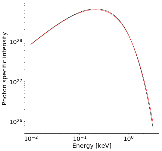
Let’s plot the spectrum and also the spectrum generated by declaring the effective gravity directly above:
[25]:
plt.figure(figsize=(8,8))

plt.plot(E, hot_I, 'k-', lw=1.0)
plt.plot(E, I_E, 'r-', lw=1.0)

ax = plt.gca()
ax.set_yscale('log')
ax.set_xscale('log')
ax.set_ylabel('Photon specific intensity')
_ = ax.set_xlabel('Energy [keV]')