Post-processing
In this tutorial we demonstrate the functionality and posterior operations supported by the PostProcessing module by operating with the example posterior samples found in examples/examples_fast/Outputs. A previous version of this Post-processing tutorial operating with the posterior samples reported by Riley et al. (2019) is given
here with more post-processing examples (however, using model files which are not supported anymore).
Initialisation
[1]:
# Importing relevant modules

%matplotlib inline

from __future__ import division

import sys
import os
import matplotlib.pyplot as plt

from matplotlib import pyplot as plt
from matplotlib import rcParams
from matplotlib.ticker import MultipleLocator, AutoLocator, AutoMinorLocator
from matplotlib import gridspec
from matplotlib import cm
from matplotlib.patches import Rectangle
import matplotlib.patches as mpatches


import warnings
warnings.simplefilter(action='ignore', category=FutureWarning)

import numpy as np
import math

from collections import OrderedDict

import xpsi

from xpsi import PostProcessing

# choose a seed for the notebook if you want caching to be useful
# and the notebook exactly reproducible
PostProcessing.set_random_seed(42)

from xpsi.global_imports import gravradius
/=============================================\
| X-PSI: X-ray Pulse Simulation and Inference |
|---------------------------------------------|
|                Version: 1.0.0               |
|---------------------------------------------|
|      https://xpsi-group.github.io/xpsi      |
\=============================================/

Imported GetDist version: 0.3.1
Imported nestcheck version: 0.2.0
[2]:
# Setting path to import additional module
path="../../examples/examples_fast/Modules/"
sys.path.append(path)
[3]:
# Importing main
import main as ST
Loading the data assuming the notebook was run for documentation pages
Setting channels for event data...
Channels set.
Setting channels for loaded instrument response (sub)matrix...
Channels set.
No parameters supplied... empty subspace created.
Creating parameter:
    > Named "phase_shift" with fixed value 0.000e+00.
    > The phase shift for the signal, a periodic parameter [cycles].
Creating parameter:
    > Named "frequency" with fixed value 3.140e+02.
    > Spin frequency [Hz].
Creating parameter:
    > Named "mass" with bounds [1.000e+00, 1.600e+00].
    > Gravitational mass [solar masses].
Creating parameter:
    > Named "radius" with bounds [1.000e+01, 1.300e+01].
    > Coordinate equatorial radius [km].
Creating parameter:
    > Named "distance" with bounds [5.000e-01, 2.000e+00].
    > Earth distance [kpc].
Creating parameter:
    > Named "cos_inclination" with bounds [0.000e+00, 1.000e+00].
    > Cosine of Earth inclination to rotation axis.
Creating parameter:
    > Named "super_colatitude" with bounds [1.000e-03, 1.570e+00].
    > The colatitude of the centre of the superseding region [radians].
Creating parameter:
    > Named "super_radius" with bounds [1.000e-03, 1.570e+00].
    > The angular radius of the (circular) superseding region [radians].
Creating parameter:
    > Named "phase_shift" with bounds [-2.500e-01, 7.500e-01].
    > The phase of the hot region, a periodic parameter [cycles].
Creating parameter:
    > Named "super_temperature" with bounds [6.000e+00, 7.000e+00].
    > log10(superseding region effective temperature [K]).
Creating parameter:
    > Named "mode_frequency" with fixed value 3.140e+02.
    > Coordinate frequency of the mode of radiative asymmetry in the
photosphere that is assumed to generate the pulsed signal [Hz].
No parameters supplied... empty subspace created.
Checking likelihood and prior evaluation before commencing sampling...
Cannot import ``allclose`` function from NumPy.
Using fallback implementation...
Checking closeness of likelihood arrays:
-4.78812782e+04 | -4.78812782e+04 .....
Closeness evaluated.
Log-likelihood value checks passed on root process.
Checks passed.
Let’s see the free parameters in our model
[4]:
ST.likelihood
[4]:
Free parameters
---------------
mass: Gravitational mass [solar masses].
radius: Coordinate equatorial radius [km].
distance: Earth distance [kpc].
cos_inclination: Cosine of Earth inclination to rotation axis.
hot__phase_shift: The phase of the hot region, a periodic parameter [cycles].
hot__super_colatitude: The colatitude of the centre of the superseding region [radians].
hot__super_radius: The angular radius of the (circular) superseding region [radians].
hot__super_temperature: log10(superseding region effective temperature [K]).
Now let’s set the names, the bounds and the labels of the free parameters for later use
[5]:
# Settings names, bounds and labels

ST.names=['mass','radius','distance','cos_inclination','hot__phase_shift',
          'hot__super_colatitude','hot__super_radius','hot__super_temperature']

# We will use the same bounds used during sampling
ST.bounds = {'mass':(1.0,1.6),
             'radius':(10,13),
             'distance':(0.5,2.0),
             'cos_inclination':(0,1),
             'hot__phase_shift':(-0.25, 0.75),
             'hot__super_colatitude':(0.001, math.pi/2 - 0.001),
             'hot__super_radius':(0.001, math.pi/2.0 - 0.001),
             'hot__super_temperature':(6., 7.)}

# Now the labels
ST.labels = {'mass': r"M\;\mathrm{[M}_{\odot}\mathrm{]}",
              'radius': r"R_{\mathrm{eq}}\;\mathrm{[km]}",
              'distance': r"D \;\mathrm{[kpc]}",
              'cos_inclination': r"\cos(i)",
              'hot__phase_shift': r"\phi_{p}\;\mathrm{[cycles]}",
              'hot__super_colatitude': r"\Theta_{spot}\;\mathrm{[rad]}",
              'hot__super_radius': r"\zeta_{spot}\;\mathrm{[rad]}",
              'hot__super_temperature': r"\mathrm{log10}(T_{spot}\;[\mathrm{K}])"}
Let’s also add the compactness because we also added that extra parameter to be derived
[6]:
ST.names +=['compactness']
ST.bounds['compactness']=(gravradius(1.0)/16.0, 1.0/3.0)
ST.labels['compactness']= r"M/R_{\mathrm{eq}}"
[7]:
# Getdist settings, usually doesn't need to be changed
getdist_kde_settings = {'ignore_rows': 0,
                         'min_weight_ratio': 1.0e-10,
                         'contours': [0.683, 0.954, 0.997],
                         'credible_interval_threshold': 0.001,
                         'range_ND_contour': 0,
                         'range_confidence': 0.001,
                         'fine_bins': 1024,
                         'smooth_scale_1D': 0.4,
                         'num_bins': 100,
                         'boundary_correction_order': 1,
                         'mult_bias_correction_order': 1,
                         'smooth_scale_2D': 0.4,
                         'max_corr_2D': 0.99,
                         'fine_bins_2D': 512,
                         'num_bins_2D': 40}
Let’s now load the run
[8]:
ST.runs = xpsi.Runs.load_runs(ID='ST',
                               run_IDs=['run'],
                               roots=['ST_live_1000_eff_0.3_seed0'],
                               base_dirs=['../../examples/examples_fast/Outputs/'],
                               use_nestcheck=[True],
                               kde_settings=getdist_kde_settings,
                               likelihood=ST.likelihood,
                               names=ST.names,
                               bounds=ST.bounds,
                               labels=ST.labels,
                               implementation='multinest',
                               overwrite_transformed=True)
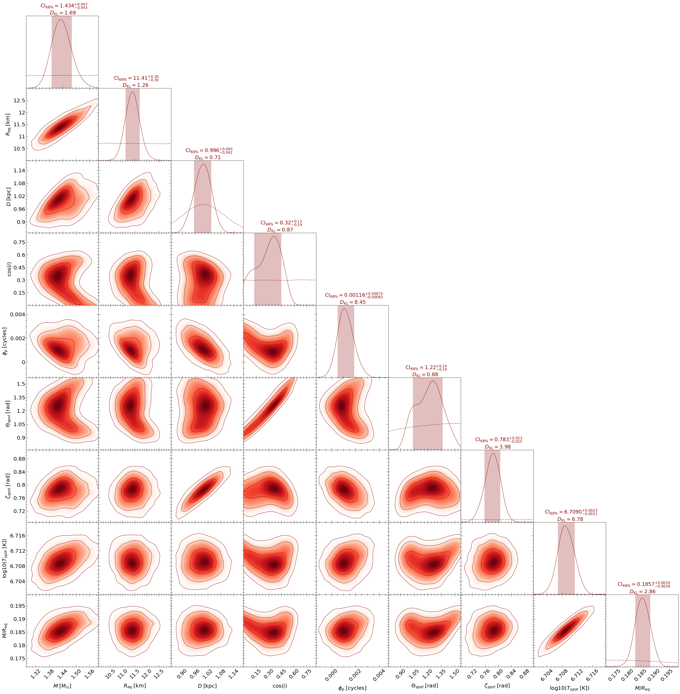
Corner plots
Let’s plot all of the inferred parameters
[9]:
pp = xpsi.PostProcessing.CornerPlotter([ST.runs])
_ = pp.plot(
     params=ST.names,
     IDs=OrderedDict([('ST', ['run',]),]),
     prior_density=True,
     KL_divergence=True,
     ndraws=5e4,
     combine=False, combine_all=True, only_combined=False, overwrite_combined=True,
     param_plot_lims={},
     bootstrap_estimators=False,
     bootstrap_density=False,
     n_simulate=200,
     crosshairs=False,
     write=False,
     ext='.png',
     maxdots=3000,
     root_filename='run',
     credible_interval_1d=True,
     annotate_credible_interval=True,
     compute_all_intervals=False,
     sixtyeight=True,
     x_label_rotation=45.0,
     num_plot_contours=3,
     subplot_size=4.0,
     legend_corner_coords=(0.675,0.8),
     legend_frameon=False,
     scale_attrs=OrderedDict([('legend_fontsize', 2.0),
                              ('lab_fontsize', 1.35),
                              ('axes_fontsize', 'lab_fontsize'),
                             ]
                            ),
     colormap='Reds',
     shaded=True,
     shade_root_index=-1,
     rasterized_shade=True,
     no_ylabel=True,
     no_ytick=True,
     lw=1.0,
     lw_1d=1.0,
     filled=False,
     normalize=True,
     veneer=True,
     #contour_colors=['orange'],
     tqdm_kwargs={'disable': False},
     lengthen=2.0,
     embolden=1.0,
     nx=500,
     scale_ymax=1.1)
Executing posterior density estimation...
Curating set of runs for posterior plotting...
Run set curated.
Constructing lower-triangle posterior density plot via Gaussian KDE:
plotting:  ['mass', 'radius']
plotting:  ['mass', 'distance']
plotting:  ['mass', 'cos_inclination']
plotting:  ['mass', 'hot__phase_shift']
plotting:  ['mass', 'hot__super_colatitude']
plotting:  ['mass', 'hot__super_radius']
plotting:  ['mass', 'hot__super_temperature']
plotting:  ['mass', 'compactness']
plotting:  ['radius', 'distance']
plotting:  ['radius', 'cos_inclination']
plotting:  ['radius', 'hot__phase_shift']
plotting:  ['radius', 'hot__super_colatitude']
plotting:  ['radius', 'hot__super_radius']
plotting:  ['radius', 'hot__super_temperature']
plotting:  ['radius', 'compactness']
plotting:  ['distance', 'cos_inclination']
plotting:  ['distance', 'hot__phase_shift']
plotting:  ['distance', 'hot__super_colatitude']
plotting:  ['distance', 'hot__super_radius']
plotting:  ['distance', 'hot__super_temperature']
plotting:  ['distance', 'compactness']
plotting:  ['cos_inclination', 'hot__phase_shift']
plotting:  ['cos_inclination', 'hot__super_colatitude']
plotting:  ['cos_inclination', 'hot__super_radius']
plotting:  ['cos_inclination', 'hot__super_temperature']
plotting:  ['cos_inclination', 'compactness']
plotting:  ['hot__phase_shift', 'hot__super_colatitude']
plotting:  ['hot__phase_shift', 'hot__super_radius']
plotting:  ['hot__phase_shift', 'hot__super_temperature']
plotting:  ['hot__phase_shift', 'compactness']
plotting:  ['hot__super_colatitude', 'hot__super_radius']
plotting:  ['hot__super_colatitude', 'hot__super_temperature']
plotting:  ['hot__super_colatitude', 'compactness']
plotting:  ['hot__super_radius', 'hot__super_temperature']
plotting:  ['hot__super_radius', 'compactness']
plotting:  ['hot__super_temperature', 'compactness']
Adding 1D marginal prior density functions...
Plotting prior for posterior ST...
Drawing samples from the joint prior...
Samples drawn.
Estimating 1D marginal KL-divergences in bits...
mass KL-divergence = 1.6920...
radius KL-divergence = 1.2603...
distance KL-divergence = 0.7114...
cos_inclination KL-divergence = 0.8743...
hot__phase_shift KL-divergence = 8.4478...
hot__super_colatitude KL-divergence = 0.8839...
hot__super_radius KL-divergence = 3.9751...
hot__super_temperature KL-divergence = 6.7775...
compactness KL-divergence = 2.8594...
Estimated 1D marginal KL-divergences.
Added 1D marginal prior density functions.
Veneering spines and axis ticks...
Veneered.
Adding 1D marginal credible intervals...
Plotting credible regions for posterior ST...
Added 1D marginal credible intervals.
Constructed lower-triangle posterior density plot.
Posterior density estimation complete.
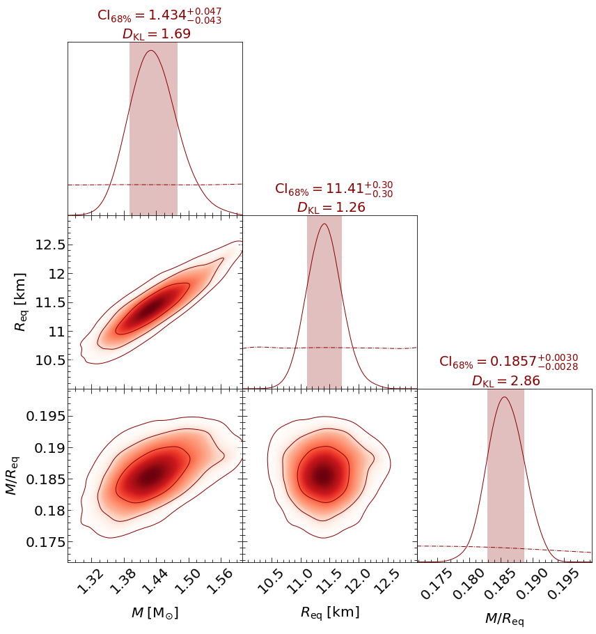
Now let’s plot a subset of those parameters, say - mass, radius and compactness
[10]:
_ = pp.plot(
     params=["mass", "radius", "compactness"],
     IDs=OrderedDict([('ST', ['run',]),]),
     prior_density=True,
     KL_divergence=True,
     ndraws=5e4,
     combine=False, combine_all=True, only_combined=False, overwrite_combined=True,
     param_plot_lims={},
     bootstrap_estimators=False,
     bootstrap_density=False,
     n_simulate=200,
     crosshairs=False,
     write=False,
     ext='.png',
     maxdots=3000,
     root_filename='run',
     credible_interval_1d=True,
     annotate_credible_interval=True,
     compute_all_intervals=False,
     sixtyeight=True,
     x_label_rotation=45.0,
     num_plot_contours=3,
     subplot_size=4.0,
     legend_corner_coords=(0.675,0.8),
     legend_frameon=False,
     scale_attrs=OrderedDict([('legend_fontsize', 2.0),
                              ('lab_fontsize', 1.35),
                              ('axes_fontsize', 'lab_fontsize'),
                             ]
                            ),
     colormap='Reds',
     shaded=True,
     shade_root_index=-1,
     rasterized_shade=True,
     no_ylabel=True,
     no_ytick=True,
     lw=1.0,
     lw_1d=1.0,
     filled=False,
     normalize=True,
     veneer=True,
     #contour_colors=['orange'],
     tqdm_kwargs={'disable': False},
     lengthen=2.0,
     embolden=1.0,
     nx=500,
     scale_ymax=1.1)
Executing posterior density estimation...
Curating set of runs for posterior plotting...
Run set curated.
Constructing lower-triangle posterior density plot via Gaussian KDE:
plotting:  ['mass', 'radius']
plotting:  ['mass', 'compactness']
plotting:  ['radius', 'compactness']
Adding 1D marginal prior density functions...
Plotting prior for posterior ST...
Drawing samples from the joint prior...
Samples drawn.
Estimating 1D marginal KL-divergences in bits...
mass KL-divergence = 1.6920...
radius KL-divergence = 1.2603...
compactness KL-divergence = 2.8594...
Estimated 1D marginal KL-divergences.
Added 1D marginal prior density functions.
Veneering spines and axis ticks...
Veneered.
Adding 1D marginal credible intervals...
Plotting credible regions for posterior ST...
Added 1D marginal credible intervals.
Constructed lower-triangle posterior density plot.
Posterior density estimation complete.
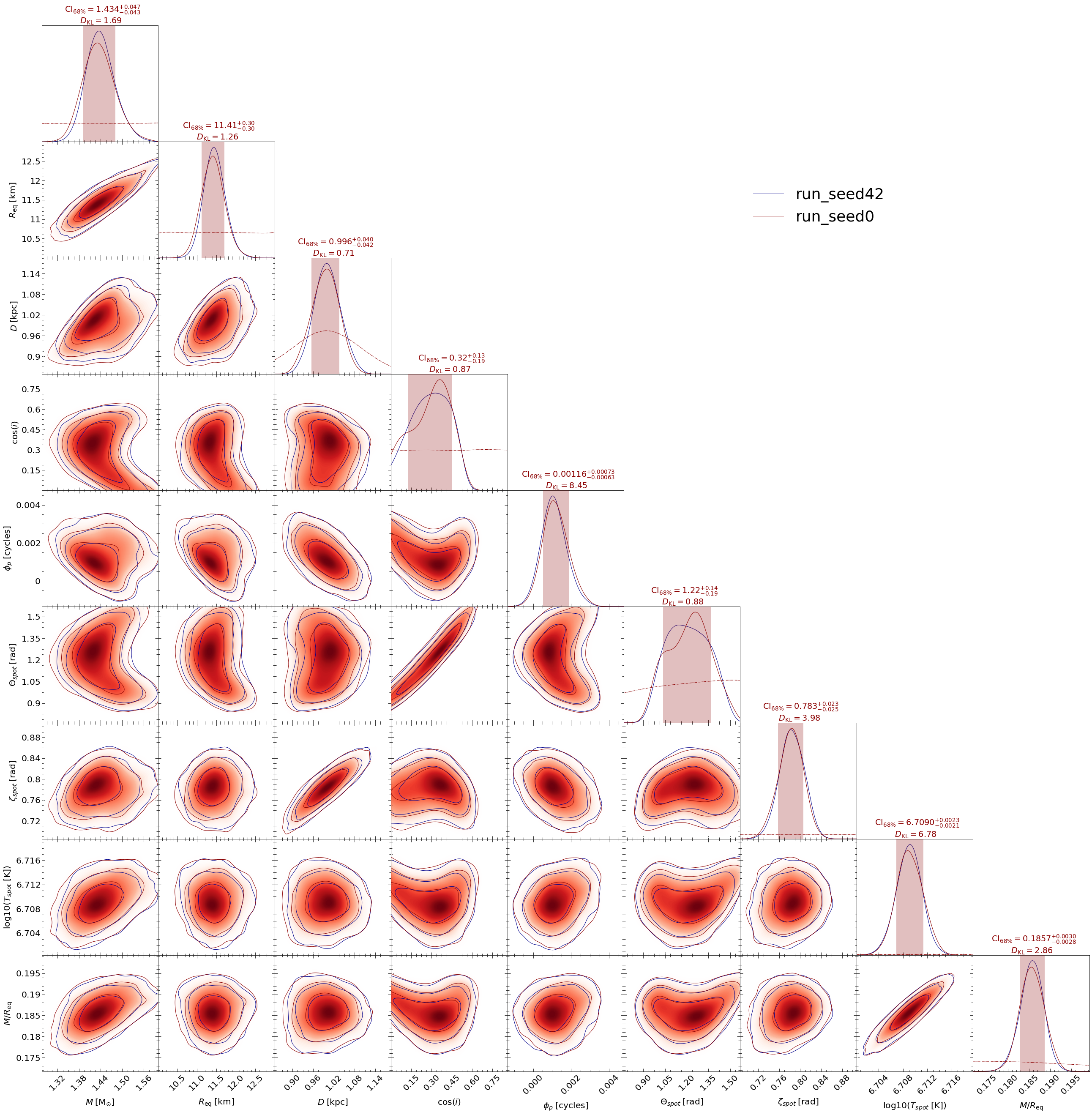
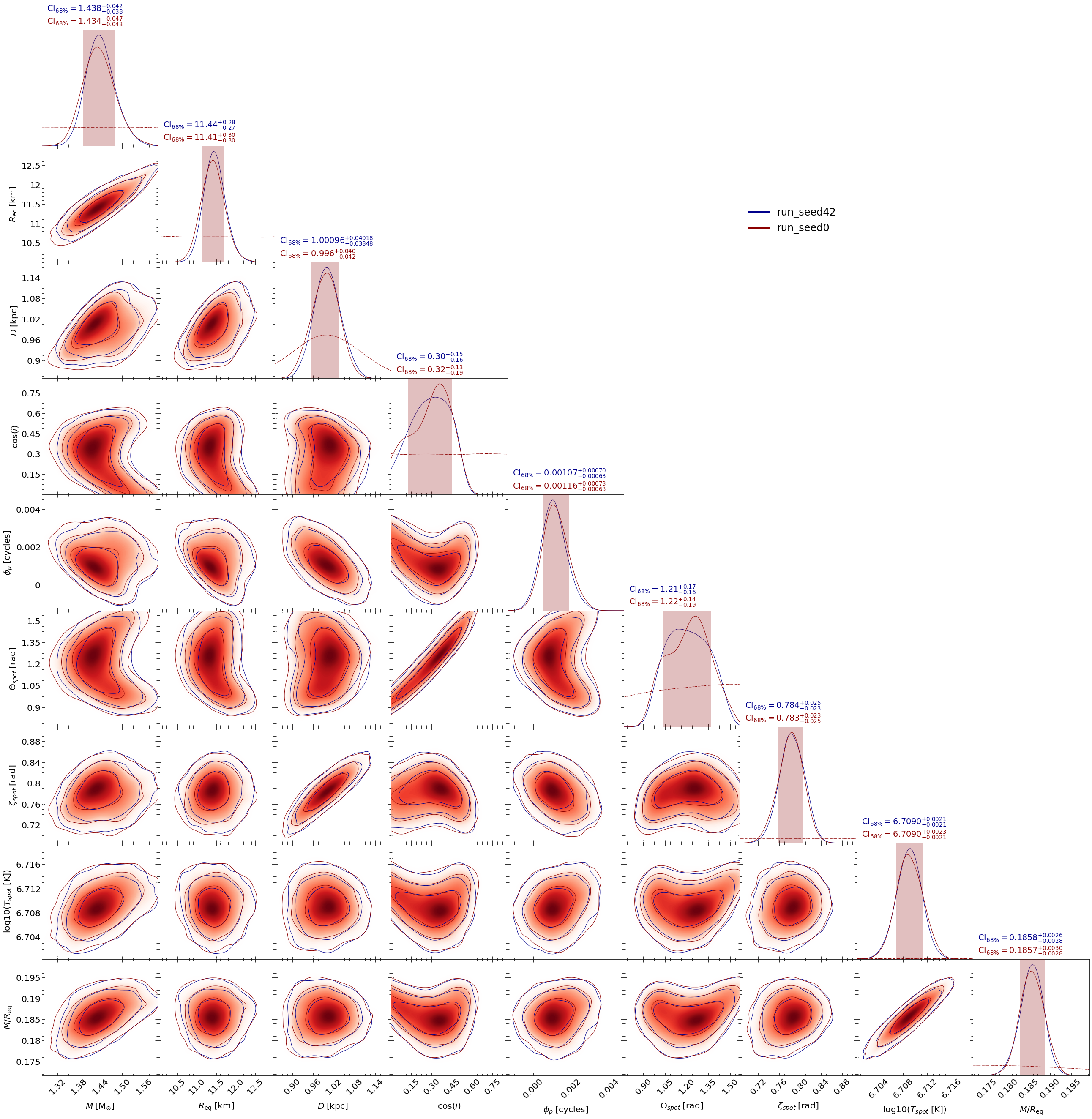
For the sake of example, let’s assume one has multiple runs for the same model and wants to plots them all on the same plot.
Here, I have two runs - one performed having fixed multinest seed to 0, and the second having fixed the seed to 42.
[11]:
# Loading the runs

ST.runs = xpsi.Runs.load_runs(ID='ST',
                               run_IDs=['run_seed0','run_seed42'],
                               roots=['ST_live_1000_eff_0.3_seed0','ST_live_1000_eff_0.3_seed42'],
                               base_dirs=['../../examples/examples_fast/Outputs/',
                                         '../../examples/examples_fast/Outputs/'],
                               use_nestcheck=[True]*2,
                               kde_settings=getdist_kde_settings,
                               likelihood=ST.likelihood,
                               names=ST.names,
                               bounds=ST.bounds,
                               labels=ST.labels,
                               implementation='multinest',
                               overwrite_transformed=True)
[12]:
# Plotting the runs

pp = xpsi.PostProcessing.CornerPlotter([ST.runs])
_ = pp.plot(
     params=ST.names,

     IDs=OrderedDict([('ST', ['run_seed0','run_seed42',]),]),
     prior_density=True,
     KL_divergence=True,
     ndraws=5e4,
     combine=False, combine_all=True, only_combined=False, overwrite_combined=True,
     param_plot_lims={},
     bootstrap_estimators=False,
     bootstrap_density=False,
     n_simulate=200,
     crosshairs=False,
     write=False,
     ext='.png',
     maxdots=3000,
     root_filename='run_all',
     credible_interval_1d=True,
     annotate_credible_interval=True,
     compute_all_intervals=False,
     sixtyeight=True,
     x_label_rotation=45.0,
     num_plot_contours=3,
     subplot_size=4.0,
     legend_corner_coords=(0.675,0.8),
     legend_frameon=False,
     scale_attrs=OrderedDict([('legend_fontsize', 3.0),
                              ('lab_fontsize', 1.35),
                              ('axes_fontsize', 'lab_fontsize'),
                             ]
                            ),
     colormap='Reds',
     shaded=True,
     shade_root_index=-1,
     rasterized_shade=True,
     no_ylabel=True,
     no_ytick=True,
     lw=1.0,
     lw_1d=1.0,
     filled=False,
     normalize=True,
     veneer=True,
     #contour_colors=['orange'],
     tqdm_kwargs={'disable': False},
     lengthen=2.0,
     embolden=1.0,
     nx=500,
     scale_ymax=1.1)
Executing posterior density estimation...
Curating set of runs for posterior plotting...
Run set curated.
Constructing lower-triangle posterior density plot via Gaussian KDE:
plotting:  ['mass', 'radius']
plotting:  ['mass', 'distance']
plotting:  ['mass', 'cos_inclination']
plotting:  ['mass', 'hot__phase_shift']
plotting:  ['mass', 'hot__super_colatitude']
plotting:  ['mass', 'hot__super_radius']
plotting:  ['mass', 'hot__super_temperature']
plotting:  ['mass', 'compactness']
plotting:  ['radius', 'distance']
plotting:  ['radius', 'cos_inclination']
plotting:  ['radius', 'hot__phase_shift']
plotting:  ['radius', 'hot__super_colatitude']
plotting:  ['radius', 'hot__super_radius']
plotting:  ['radius', 'hot__super_temperature']
plotting:  ['radius', 'compactness']
plotting:  ['distance', 'cos_inclination']
plotting:  ['distance', 'hot__phase_shift']
plotting:  ['distance', 'hot__super_colatitude']
plotting:  ['distance', 'hot__super_radius']
plotting:  ['distance', 'hot__super_temperature']
plotting:  ['distance', 'compactness']
plotting:  ['cos_inclination', 'hot__phase_shift']
plotting:  ['cos_inclination', 'hot__super_colatitude']
plotting:  ['cos_inclination', 'hot__super_radius']
plotting:  ['cos_inclination', 'hot__super_temperature']
plotting:  ['cos_inclination', 'compactness']
plotting:  ['hot__phase_shift', 'hot__super_colatitude']
plotting:  ['hot__phase_shift', 'hot__super_radius']
plotting:  ['hot__phase_shift', 'hot__super_temperature']
plotting:  ['hot__phase_shift', 'compactness']
plotting:  ['hot__super_colatitude', 'hot__super_radius']
plotting:  ['hot__super_colatitude', 'hot__super_temperature']
plotting:  ['hot__super_colatitude', 'compactness']
plotting:  ['hot__super_radius', 'hot__super_temperature']
plotting:  ['hot__super_radius', 'compactness']
plotting:  ['hot__super_temperature', 'compactness']
Adding 1D marginal prior density functions...
Plotting prior for posterior ST...
Drawing samples from the joint prior...
Samples drawn.
Estimating 1D marginal KL-divergences in bits...
mass KL-divergence = 1.6920...
radius KL-divergence = 1.2603...
distance KL-divergence = 0.7114...
cos_inclination KL-divergence = 0.8743...
hot__phase_shift KL-divergence = 8.4478...
hot__super_colatitude KL-divergence = 0.8839...
hot__super_radius KL-divergence = 3.9751...
hot__super_temperature KL-divergence = 6.7775...
compactness KL-divergence = 2.8594...
Estimated 1D marginal KL-divergences.
Added 1D marginal prior density functions.
Veneering spines and axis ticks...
Veneered.
Adding 1D marginal credible intervals...
Plotting credible regions for posterior ST...
Added 1D marginal credible intervals.
Constructed lower-triangle posterior density plot.
Posterior density estimation complete.
In the previous plot, on the credible interval of the first run id is shown, let’s now show all of them.
[13]:
pp = xpsi.PostProcessing.CornerPlotter([ST.runs])
_ = pp.plot(
     params=ST.names,

     IDs=OrderedDict([('ST', ['run_seed0','run_seed42',]),]),
     prior_density=True,
     KL_divergence=True,
     ndraws=5e4,
     combine=False, combine_all=True, only_combined=False, overwrite_combined=True,
     param_plot_lims={},
     bootstrap_estimators=False,
     bootstrap_density=False,
     n_simulate=200,
     crosshairs=True, # Turn this to true
     write=False,
     ext='.png',
     maxdots=3000,
     root_filename='run',
     credible_interval_1d=True,
     credible_interval_1d_all_show=True, # Turn this to true
     annotate_credible_interval=True,
     compute_all_intervals=False,
     sixtyeight=True,
     x_label_rotation=45.0,
     num_plot_contours=3,
     subplot_size=4.0,
     legend_corner_coords=(0.675,0.8),
     legend_frameon=False,
     scale_attrs=OrderedDict([('legend_fontsize', 2.0),
                              ('lab_fontsize', 1.35),
                              ('axes_fontsize', 'lab_fontsize'),
                             ]
                            ),
     colormap='Reds',
     shaded=True,
     shade_root_index=-1,
     rasterized_shade=True,
     no_ylabel=True,
     no_ytick=True,
     lw=1.0,
     lw_1d=1.0,
     filled=False,
     normalize=True,
     veneer=True,
     #contour_colors=['orange'],
     tqdm_kwargs={'disable': False},
     lengthen=2.0,
     embolden=1.0,
     nx=500 ,
    scale_ymax=1.1)
Executing posterior density estimation...
Curating set of runs for posterior plotting...
Run set curated.
Constructing lower-triangle posterior density plot via Gaussian KDE:
plotting:  ['mass', 'radius']
plotting:  ['mass', 'distance']
plotting:  ['mass', 'cos_inclination']
plotting:  ['mass', 'hot__phase_shift']
plotting:  ['mass', 'hot__super_colatitude']
plotting:  ['mass', 'hot__super_radius']
plotting:  ['mass', 'hot__super_temperature']
plotting:  ['mass', 'compactness']
plotting:  ['radius', 'distance']
plotting:  ['radius', 'cos_inclination']
plotting:  ['radius', 'hot__phase_shift']
plotting:  ['radius', 'hot__super_colatitude']
plotting:  ['radius', 'hot__super_radius']
plotting:  ['radius', 'hot__super_temperature']
plotting:  ['radius', 'compactness']
plotting:  ['distance', 'cos_inclination']
plotting:  ['distance', 'hot__phase_shift']
plotting:  ['distance', 'hot__super_colatitude']
plotting:  ['distance', 'hot__super_radius']
plotting:  ['distance', 'hot__super_temperature']
plotting:  ['distance', 'compactness']
plotting:  ['cos_inclination', 'hot__phase_shift']
plotting:  ['cos_inclination', 'hot__super_colatitude']
plotting:  ['cos_inclination', 'hot__super_radius']
plotting:  ['cos_inclination', 'hot__super_temperature']
plotting:  ['cos_inclination', 'compactness']
plotting:  ['hot__phase_shift', 'hot__super_colatitude']
plotting:  ['hot__phase_shift', 'hot__super_radius']
plotting:  ['hot__phase_shift', 'hot__super_temperature']
plotting:  ['hot__phase_shift', 'compactness']
plotting:  ['hot__super_colatitude', 'hot__super_radius']
plotting:  ['hot__super_colatitude', 'hot__super_temperature']
plotting:  ['hot__super_colatitude', 'compactness']
plotting:  ['hot__super_radius', 'hot__super_temperature']
plotting:  ['hot__super_radius', 'compactness']
plotting:  ['hot__super_temperature', 'compactness']
Adding 1D marginal prior density functions...
Plotting prior for posterior ST...
Drawing samples from the joint prior...
Samples drawn.
Added 1D marginal prior density functions.
Veneering spines and axis ticks...
Veneered.
Adding parameter truth crosshairs...
Added crosshairs.
Adding 1D marginal credible intervals...
Plotting credible regions for posterior ST...
Added 1D marginal credible intervals.
Adding 1D marginal credible intervals...
Plotting credible regions for posterior ST...
Added 1D marginal credible intervals.
Constructed lower-triangle posterior density plot.
Posterior density estimation complete.

Let’s now make the legend line width a bit bigger
[14]:
pp = xpsi.PostProcessing.CornerPlotter([ST.runs])
_ = pp.plot(
     params=ST.names,

     IDs=OrderedDict([('ST', ['run_seed0','run_seed42',]),]),
     prior_density=True,
     KL_divergence=True,
     ndraws=5e4,
     combine=False, combine_all=True, only_combined=False, overwrite_combined=True,
     param_plot_lims={},
     bootstrap_estimators=False,
     bootstrap_density=False,
     n_simulate=200,
     crosshairs=True, # Turn this to true
     write=False,
     ext='.png',
     maxdots=3000,
     root_filename='run',
     credible_interval_1d=True,
     credible_interval_1d_all_show=True, # Turn this to true
     annotate_credible_interval=True,
     compute_all_intervals=False,
     sixtyeight=True,
     x_label_rotation=45.0,
     num_plot_contours=3,
     subplot_size=4.0,
     legend_corner_coords=(0.675,0.8),
     legend_frameon=False,
     scale_attrs=OrderedDict([('legend_fontsize', 2.0),
                              ('lab_fontsize', 1.35),
                              ('axes_fontsize', 'lab_fontsize'),
                             ]
                            ),
     colormap='Reds',
     shaded=True,
     shade_root_index=-1,
     rasterized_shade=True,
     no_ylabel=True,
     no_ytick=True,
     lw=1.0,
     lw_1d=1.0,
     filled=False,
     normalize=True,
     veneer=True,
     #contour_colors=['orange'],
     tqdm_kwargs={'disable': False},
     lengthen=2.0,
     embolden=1.0,
     nx=500 ,
    scale_ymax=1.1)


 # If you have multiple runs/models, you can increase the legend linewidth
for legobj in _.legend.legendHandles:
        legobj.set_linewidth(5.0)
Executing posterior density estimation...
Curating set of runs for posterior plotting...
Run set curated.
Constructing lower-triangle posterior density plot via Gaussian KDE:
plotting:  ['mass', 'radius']
plotting:  ['mass', 'distance']
plotting:  ['mass', 'cos_inclination']
plotting:  ['mass', 'hot__phase_shift']
plotting:  ['mass', 'hot__super_colatitude']
plotting:  ['mass', 'hot__super_radius']
plotting:  ['mass', 'hot__super_temperature']
plotting:  ['mass', 'compactness']
plotting:  ['radius', 'distance']
plotting:  ['radius', 'cos_inclination']
plotting:  ['radius', 'hot__phase_shift']
plotting:  ['radius', 'hot__super_colatitude']
plotting:  ['radius', 'hot__super_radius']
plotting:  ['radius', 'hot__super_temperature']
plotting:  ['radius', 'compactness']
plotting:  ['distance', 'cos_inclination']
plotting:  ['distance', 'hot__phase_shift']
plotting:  ['distance', 'hot__super_colatitude']
plotting:  ['distance', 'hot__super_radius']
plotting:  ['distance', 'hot__super_temperature']
plotting:  ['distance', 'compactness']
plotting:  ['cos_inclination', 'hot__phase_shift']
plotting:  ['cos_inclination', 'hot__super_colatitude']
plotting:  ['cos_inclination', 'hot__super_radius']
plotting:  ['cos_inclination', 'hot__super_temperature']
plotting:  ['cos_inclination', 'compactness']
plotting:  ['hot__phase_shift', 'hot__super_colatitude']
plotting:  ['hot__phase_shift', 'hot__super_radius']
plotting:  ['hot__phase_shift', 'hot__super_temperature']
plotting:  ['hot__phase_shift', 'compactness']
plotting:  ['hot__super_colatitude', 'hot__super_radius']
plotting:  ['hot__super_colatitude', 'hot__super_temperature']
plotting:  ['hot__super_colatitude', 'compactness']
plotting:  ['hot__super_radius', 'hot__super_temperature']
plotting:  ['hot__super_radius', 'compactness']
plotting:  ['hot__super_temperature', 'compactness']
Adding 1D marginal prior density functions...
Plotting prior for posterior ST...
Drawing samples from the joint prior...
Samples drawn.
Added 1D marginal prior density functions.
Veneering spines and axis ticks...
Veneered.
Adding parameter truth crosshairs...
Added crosshairs.
Adding 1D marginal credible intervals...
Plotting credible regions for posterior ST...
Added 1D marginal credible intervals.
Adding 1D marginal credible intervals...
Plotting credible regions for posterior ST...
Added 1D marginal credible intervals.
Constructed lower-triangle posterior density plot.
Posterior density estimation complete.
We can also obtain the credible intervals shown on the plots in the form of a list
[15]:
credible_intervals=pp.credible_intervals
[16]:
# Printing the first one:
print(credible_intervals["ST_run_seed0"])
[[ 1.434e+00 -4.300e-02  4.700e-02]
 [ 1.141e+01 -3.000e-01  3.000e-01]
 [ 9.960e-01 -4.200e-02  4.000e-02]
 [ 3.200e-01 -1.900e-01  1.300e-01]
 [ 1.160e-03 -6.300e-04  7.300e-04]
 [ 1.220e+00 -1.900e-01  1.400e-01]
 [ 7.830e-01 -2.500e-02  2.300e-02]
 [ 6.709e+00 -2.100e-03  2.300e-03]
 [ 1.857e-01 -2.800e-03  3.000e-03]]
[17]:
# Printing the second one:
print(credible_intervals["ST_run_seed42"])
[[ 1.43800e+00 -3.80000e-02  4.20000e-02]
 [ 1.14400e+01 -2.70000e-01  2.80000e-01]
 [ 1.00096e+00 -3.84800e-02  4.01800e-02]
 [ 3.00000e-01 -1.60000e-01  1.50000e-01]
 [ 1.07000e-03 -6.30000e-04  7.00000e-04]
 [ 1.21000e+00 -1.60000e-01  1.70000e-01]
 [ 7.84000e-01 -2.30000e-02  2.50000e-02]
 [ 6.70900e+00 -2.10000e-03  2.10000e-03]
 [ 1.85800e-01 -2.80000e-03  2.60000e-03]]
Assuming that one knows the values that have been used to produce the data and wants to show them:
[18]:
# In our case:

ST.truths={'mass': 1.4,                               # Mass in solar Mass
          'radius': 12.,                              # Equatorial radius in km
          'distance': 1.0,                            # Distance in kpc
          'cos_inclination': math.cos(60*np.pi/180),  # Cosine of Earth inclination to rotation axis
          'hot__phase_shift': 0.0,                    # Phase shift
          'hot__super_colatitude': 70*np.pi/180,      # Colatitude of the centre of the superseding region
          'hot__super_radius': 0.75,                  # Angular radius of the (circular) superseding region
          'hot__super_temperature':6.7}               # Temperature in log

ST.truths['compactness']=gravradius(ST.truths['mass'])/ST.truths['radius']
[19]:
# Loading the run again :)

ST.runs = xpsi.Runs.load_runs(ID='ST',
                               run_IDs=['run'],
                               roots=['ST_live_1000_eff_0.3_seed0'],
                               base_dirs=['../../examples/examples_fast/Outputs/'],
                               use_nestcheck=[True],
                               kde_settings=getdist_kde_settings,
                               likelihood=ST.likelihood,
                               names=ST.names,
                               bounds=ST.bounds,
                               labels=ST.labels,
                               truths=ST.truths, # Adding this line
                               implementation='multinest',
                               overwrite_transformed=True)
[20]:
pp = xpsi.PostProcessing.CornerPlotter([ST.runs])
_ = pp.plot(
     params=ST.names,

     IDs=OrderedDict([('ST', ['run',]),]),
     prior_density=True,
     KL_divergence=True,
     ndraws=5e4,
     combine=False, combine_all=True, only_combined=False, overwrite_combined=True,
     param_plot_lims={},
     bootstrap_estimators=False,
     bootstrap_density=False,
     n_simulate=200,
     crosshairs=True, # Turn this to true
     write=False,
     ext='.png',
     maxdots=3000,
     root_filename='run',
     credible_interval_1d=True,
     credible_interval_1d_show_all=True,
     annotate_credible_interval=True,
     compute_all_intervals=False,
     sixtyeight=True,
     x_label_rotation=45.0,
     num_plot_contours=3,
     subplot_size=4.0,
     legend_corner_coords=(0.675,0.8),
     legend_frameon=False,
     scale_attrs=OrderedDict([('legend_fontsize', 2.0),
                              ('lab_fontsize', 1.35),
                              ('axes_fontsize', 'lab_fontsize'),
                             ]
                            ),
     colormap='Reds',
     shaded=True,
     shade_root_index=-1,
     rasterized_shade=True,
     no_ylabel=True,
     no_ytick=True,
     lw=1.0,
     lw_1d=1.0,
     filled=False,
     normalize=True,
     veneer=True,
     #contour_colors=['orange'],
     tqdm_kwargs={'disable': False},
     lengthen=2.0,
     embolden=1.0,
     nx=500 ,
    scale_ymax=1.1)
Executing posterior density estimation...
Curating set of runs for posterior plotting...
Run set curated.
Constructing lower-triangle posterior density plot via Gaussian KDE:
plotting:  ['mass', 'radius']
plotting:  ['mass', 'distance']
plotting:  ['mass', 'cos_inclination']
plotting:  ['mass', 'hot__phase_shift']
plotting:  ['mass', 'hot__super_colatitude']
plotting:  ['mass', 'hot__super_radius']
plotting:  ['mass', 'hot__super_temperature']
plotting:  ['mass', 'compactness']
plotting:  ['radius', 'distance']
plotting:  ['radius', 'cos_inclination']
plotting:  ['radius', 'hot__phase_shift']
plotting:  ['radius', 'hot__super_colatitude']
plotting:  ['radius', 'hot__super_radius']
plotting:  ['radius', 'hot__super_temperature']
plotting:  ['radius', 'compactness']
plotting:  ['distance', 'cos_inclination']
plotting:  ['distance', 'hot__phase_shift']
plotting:  ['distance', 'hot__super_colatitude']
plotting:  ['distance', 'hot__super_radius']
plotting:  ['distance', 'hot__super_temperature']
plotting:  ['distance', 'compactness']
plotting:  ['cos_inclination', 'hot__phase_shift']
plotting:  ['cos_inclination', 'hot__super_colatitude']
plotting:  ['cos_inclination', 'hot__super_radius']
plotting:  ['cos_inclination', 'hot__super_temperature']
plotting:  ['cos_inclination', 'compactness']
plotting:  ['hot__phase_shift', 'hot__super_colatitude']
plotting:  ['hot__phase_shift', 'hot__super_radius']
plotting:  ['hot__phase_shift', 'hot__super_temperature']
plotting:  ['hot__phase_shift', 'compactness']
plotting:  ['hot__super_colatitude', 'hot__super_radius']
plotting:  ['hot__super_colatitude', 'hot__super_temperature']
plotting:  ['hot__super_colatitude', 'compactness']
plotting:  ['hot__super_radius', 'hot__super_temperature']
plotting:  ['hot__super_radius', 'compactness']
plotting:  ['hot__super_temperature', 'compactness']
Adding 1D marginal prior density functions...
Plotting prior for posterior ST...
Drawing samples from the joint prior...
Samples drawn.
Estimating 1D marginal KL-divergences in bits...
mass KL-divergence = 1.6920...
radius KL-divergence = 1.2603...
distance KL-divergence = 0.7114...
cos_inclination KL-divergence = 0.8743...
hot__phase_shift KL-divergence = 8.4478...
hot__super_colatitude KL-divergence = 0.8839...
hot__super_radius KL-divergence = 3.9751...
hot__super_temperature KL-divergence = 6.7775...
compactness KL-divergence = 2.8594...
Estimated 1D marginal KL-divergences.
Added 1D marginal prior density functions.
Veneering spines and axis ticks...
Veneered.
Adding parameter truth crosshairs...
Added crosshairs.
Adding 1D marginal credible intervals...
Plotting credible regions for posterior ST...
Added 1D marginal credible intervals.
Constructed lower-triangle posterior density plot.
Posterior density estimation complete.

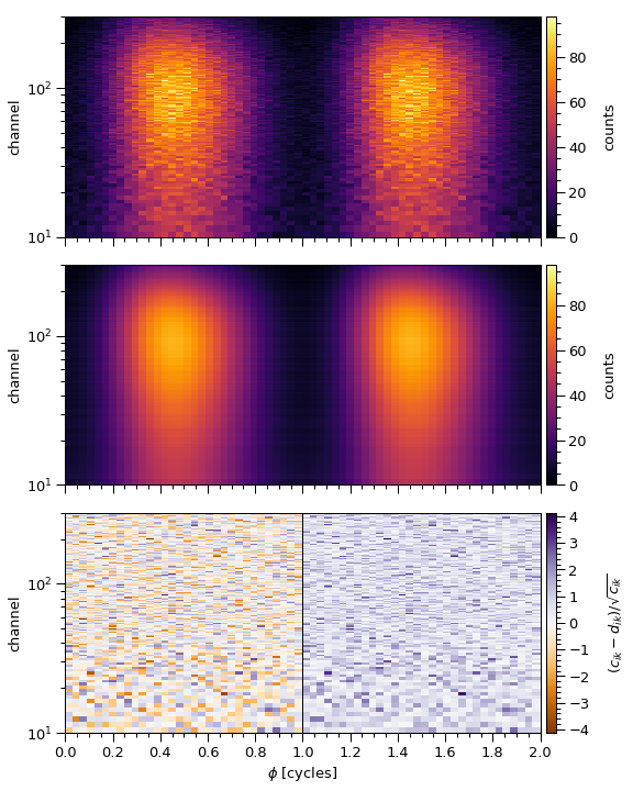
Residual plot
Now let’s plot the standardised Poissonian residuals of the first run
[21]:
pp = xpsi.SignalPlotter([ST.runs])
pp.plot(IDs=OrderedDict([('ST', ['run']),
                        ]),
        combine=False, # use these controls if more than one run for a posterior
        combine_all=False,
        force_combine=False,
        only_combined=False,
        force_cache=True,
        nsamples=100,
        plots = {'ST': xpsi.ResidualPlot()})

pp.plots["ST"].fig
Instantiating a residual plotter for posterior checking...
Declaring plot class settings...
Settings declared.
Residual plotter instantiated.
Plotting signals for posterior checking...
Curating set of runs for posterior plotting...
Run set curated.
Handling posterior ST...
Checking whether an existing cache can be read:
Creating new cache file...
Initialising cache file...
Cache file initialised.
Cache file created.
Cache state determined.
ResidualPlot object iterating over samples...
ResidualPlot object finished iterating.
ResidualPlot object finalizing...
ResidualPlot object finalized.
Writing plot to disk...
ResidualPlot instance plot will be written to path ./ST.run__signalplot_residuals.pdf...
Written.
Handled posterior ST.
Plotted signals for posterior checking.
[21]: